Count Coloured cells

baileyb103

New Member
Joined
Jan 16, 2023
Messages
22
Office Version
  1. 365
Platform
  1. Windows
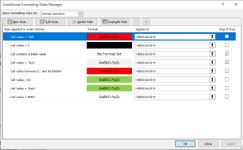
Hi. I have a spreadsheet for some assessment results (See my other posts). the cells are condition formatted so that they turn red when the assessment has failed. I am trying to get a formula to count the cells that have turned red, for each individual trainee, however the normal count functions don't seem to work with conditional formatted colours. Is there anything else I could do other than just manually in-puting the figures? The document is uploaded to a Sharepoint so would a VBA work if someone else opened the document via the Sharepoint (my knowledge on VBA is practically nothing).

Many thanks in advance.
 

Excel Facts

Did you know Excel offers Filter by Selection?
Add the AutoFilter icon to the Quick Access Toolbar. Select a cell containing Apple, click AutoFilter, and you will get all rows with Apple
Hi, what is the conditional formatting rule? You could probably use the same logic in a COUNTIFS() formula.
I have used =COUNTIF(B3:AO3, "Red"), however this doesn't seem to work if the cells are coloured via conditional formatting.
 
Upvote 0
Hi, what does your conditional formatting rule look like? Are you using the "Use a formula" method, or "Formal only cells that contain" or something else?

Please post the full details of the rule.
 
Upvote 0
Hi, what does your conditional formatting rule look like? Are you using the "Use a formula" method, or "Formal only cells that contain" or something else?

Please post the full details of the rule.
 

Attachments

  • excel.PNG
    excel.PNG
    32.6 KB · Views: 13
Upvote 0
If it's just the ones being formatted by the first rule that you are trying to count, then you can try:

Excel Formula:
=COUNTIFS(B3:AO3, "Fail")
 
Upvote 0
If it's just the ones being formatted by the first rule that you are trying to count, then you can try:

Excel Formula:
=COUNTIFS(B3:AO3, "Fail")
It would be the 'Fails', and between 0.1 and 64.99999, as some are practicals (pass or Fail) and some are % where 65% is the pass mark.
 
Upvote 0
From the looks of your screen shot, your %'s aren't formatted as %'s - try this subtle change instead.

Excel Formula:
=COUNTIFS(B3:AO3, "Fail") + COUNTIFS(B3:AO3, ">0",B3:AO3,"<65")
 
Upvote 0
Solution

Forum statistics

Threads
1,215,071
Messages
6,122,963
Members
449,094
Latest member
Anshu121

We've detected that you are using an adblocker.

We have a great community of people providing Excel help here, but the hosting costs are enormous. You can help keep this site running by allowing ads on MrExcel.com.
Allow Ads at MrExcel

Which adblocker are you using?

Disable AdBlock

Follow these easy steps to disable AdBlock

1)Click on the icon in the browser’s toolbar.
2)Click on the icon in the browser’s toolbar.
2)Click on the "Pause on this site" option.
Go back

Disable AdBlock Plus

Follow these easy steps to disable AdBlock Plus

1)Click on the icon in the browser’s toolbar.
2)Click on the toggle to disable it for "mrexcel.com".
Go back

Disable uBlock Origin

Follow these easy steps to disable uBlock Origin

1)Click on the icon in the browser’s toolbar.
2)Click on the "Power" button.
3)Click on the "Refresh" button.
Go back

Disable uBlock

Follow these easy steps to disable uBlock

1)Click on the icon in the browser’s toolbar.
2)Click on the "Power" button.
3)Click on the "Refresh" button.
Go back
Back
Top