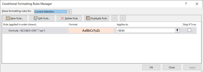
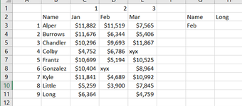
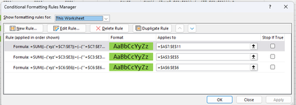
Conditional formatting formula for Highlighting a row that contains either xyx or blank cell

[nsa1]

Need help with conditional formatting formula and apply for highlighting a row that contains either text "xyx" or blank cell/cells

see below snapshots...

thanks,
NA

 

[awoohaw]

try this:

Mr excel questions 53.xlsm
	A	B	C	D	E	F	G	H	I	J
1			1	2	3
2		Name	Jan	Feb	Mar		Name	Long	CF Rule	CF Rule Text
3	1	Alper	8711	9912	5981				FALSE	=SUM((--("xyz"=$C3:$E3))+(--(""=$C3:$E3)))>0
4	2	Burrows	7577	11930	9924				FALSE
5	3	Chandler	10310	10790	9763				FALSE
6	4	Colby	10290	10335	xyz				TRUE
7	5	Frantz	10815	6272	7561				FALSE
8	6	Gonzalez	7001	xyz	7806				TRUE
9	7	Kyle	11854	8288	8432				FALSE
10	8	Little	6409		10608				TRUE
11	9	Long	6132	5104	8439				FALSE
nsa1

Cell Formulas
Range	Formula
A3:A11	A3	=SEQUENCE(9)
J3	J3	=FORMULATEXT(I3)
I3:I11	I3	=SUM((--("xyz"=$C3:$E3))+(--(""=$C3:$E3)))>0
Dynamic array formulas.

Cells with Conditional Formatting
Cell	Condition		Cell Format	Stop If True
A7:E11	Expression	=SUM((--("xyz"=$C7:$E7))+(--(""=$C7:$E7)))>0	text	NO
A3:E5	Expression	=SUM((--("xyz"=$C3:$E3))+(--(""=$C3:$E3)))>0	text	NO
A6:E6	Expression	=SUM((--("xyz"=$C6:$E6))+(--(""=$C6:$E6)))>0	text	NO

 

[nsa1]

thanks. I am wondering why do we need to input three separate rules in formula?

Is your response to have all Conditional Formatting Formulas or Cell Formulas?

 

[nsa1]

Why Three formulas for Conditional Formatting? I need to have this dynamic...where if anytime cell value changes to xyz or blank (range C3:E11) then have that row highlighted

 

[Fluff]

How about

Fluff.xlsm
	A	B	C	D	E
1
2		Name	Jan	Feb	Mar
3	1	Alper	8711	9912	5981
4	2	Burrows	7577	11930	9924
5	3	Chandler	10310	10790	9763
6	4	Colby	10290	10335	xyz
7	5	Frantz	10815	6272	7561
8	6	Gonzalez	7001	xyz	7806
9	7	Kyle	11854	8288	8432
10	8	Little	6409		10608
11	9	Long	6132	5104	8439
12
13
Master

Cells with Conditional Formatting
Cell	Condition		Cell Format	Stop If True
A3:E20	Expression	=AND($A3<>"",OR(COUNTIFS($C3:$E3,"xyz"),COUNTIFS($C3:$E3,"")))	text	NO

 

[nsa1]

Thanks so much!

 

[Fluff]

Glad we could help & thanks for the feedback.

 

[awoohaw]

Why Three formulas for Conditional Formatting? I need to have this dynamic...where if anytime cell value changes to xyz or blank (range C3:E11) then have that row highlighted

It isn't really 3 formulas. When I first built the worksheet I copied the CF to two additional sections.
I did a center row first, then the section above that and then the bottom section.

I realized that and posted a picture with only 1 formula, but I forgot to repost an xl2bb. I regret the confusion.

 

[nsa1]

It isn't really 3 formulas. When I first built the worksheet I copied the CF to two additional sections.
I did a center row first, then the section above that and then the bottom section.

I realized that and posted a picture with only 1 formula, but I forgot to repost an xl2bb. I regret the confusion.

One of the problem I came across was if blank cell was replaced by number then the highlight goes away as expected but if I type a characters (ie xyx) then the highlight remains. I only want it to highlight the row if it contains blank cell.

NA

 

[awoohaw]

One of the problem I came across was if blank cell was replaced by number then the highlight goes away as expected but if I type a characters (ie xyx) then the highlight remains. I only want it to highlight the row if it contains blank cell.

NA

I'm not sure what you mean.... here is the original data with conditional formatting:

Mr excel questions 53.xlsm
	A	B	C	D	E	F	G	H	I	J
1			1	2	3
2		Name	Jan	Feb	Mar		Name	Long	CF Rule	CF Rule Text
3	1	Alper	8711	9912	5981				FALSE	=SUM((--("xyz"=$C3:$E3))+(--(""=$C3:$E3)))>0
4	2	Burrows	7577	11930	9924				FALSE
5	3	Chandler	10310	10790	9763				FALSE
6	4	Colby		10335	xyz				TRUE
7	5	Frantz	10815	6272	7561				FALSE
8	6	Gonzalez	7001	xyz	7806				TRUE
9	7	Kyle	11854	8288	8432				FALSE
10	8	Little	6409		10608				TRUE
11	9	Long	6132	5104	8439				FALSE
nsa1

Cell Formulas
Range	Formula
J3	J3	=FORMULATEXT(I3)
I3:I11	I3	=SUM((--("xyz"=$C3:$E3))+(--(""=$C3:$E3)))>0

Cells with Conditional Formatting
Cell	Condition		Cell Format	Stop If True
A3:E11	Expression	=SUM((--("xyz"=$C3:$E3))+(--(""=$C3:$E3)))>0	text	NO

Here is when I put a value in cell D10:
(Note that the conditional formatting rule does not activate)

Mr excel questions 53.xlsm
	A	B	C	D	E	F	G	H	I	J
1			1	2	3
2		Name	Jan	Feb	Mar		Name	Long	CF Rule	CF Rule Text
3	1	Alper	8711	9912	5981				FALSE	=SUM((--("xyz"=$C3:$E3))+(--(""=$C3:$E3)))>0
4	2	Burrows	7577	11930	9924				FALSE
5	3	Chandler	10310	10790	9763				FALSE
6	4	Colby		10335	xyz				TRUE
7	5	Frantz	10815	6272	7561				FALSE
8	6	Gonzalez	7001	xyz	7806				TRUE
9	7	Kyle	11854	8288	8432				FALSE
10	8	Little	6409	4654	10608				FALSE
11	9	Long	6132	5104	8439				FALSE
nsa1

Cell Formulas
Range	Formula
J3	J3	=FORMULATEXT(I3)
I3:I11	I3	=SUM((--("xyz"=$C3:$E3))+(--(""=$C3:$E3)))>0