-
If you would like to post, please check out the MrExcel Message Board FAQ and register here. If you forgot your password, you can reset your password.
You are using an out of date browser. It may not display this or other websites correctly.
You should upgrade or use an alternative browser.
You should upgrade or use an alternative browser.
Conditional formatting formula for Highlighting a row that contains either xyx or blank cell
- Thread starter nsa1
- Start date
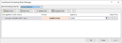
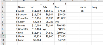
As you can see in your example...row#8 has no blank cell and only "xyx" but it still highlights...when it shouldn't...I only want it highlighted when there is empty cell in a rowI'm not sure what you mean.... here is the original data with conditional formatting:
Mr excel questions 53.xlsm
A B C D E F G H I J 1 1 2 3 2 Name Jan Feb Mar Name Long CF Rule CF Rule Text 3 1 Alper 8711 9912 5981 FALSE =SUM((--("xyz"=$C3:$E3))+(--(""=$C3:$E3)))>0 4 2 Burrows 7577 11930 9924 FALSE 5 3 Chandler 10310 10790 9763 FALSE 6 4 Colby 10335 xyz TRUE 7 5 Frantz 10815 6272 7561 FALSE 8 6 Gonzalez 7001 xyz 7806 TRUE 9 7 Kyle 11854 8288 8432 FALSE 10 8 Little 6409 10608 TRUE 11 9 Long 6132 5104 8439 FALSE
Cell Formulas Range Formula J3 J3 =FORMULATEXT(I3) I3:I11 I3 =SUM((--("xyz"=$C3:$E3))+(--(""=$C3:$E3)))>0
Cells with Conditional Formatting Cell Condition Cell Format Stop If True A3:E11 Expression =SUM((--("xyz"=$C3:$E3))+(--(""=$C3:$E3)))>0 text NO
Here is when I put a value in cell D10:
(Note that the conditional formatting rule does not activate)
Mr excel questions 53.xlsm
A B C D E F G H I J 1 1 2 3 2 Name Jan Feb Mar Name Long CF Rule CF Rule Text 3 1 Alper 8711 9912 5981 FALSE =SUM((--("xyz"=$C3:$E3))+(--(""=$C3:$E3)))>0 4 2 Burrows 7577 11930 9924 FALSE 5 3 Chandler 10310 10790 9763 FALSE 6 4 Colby 10335 xyz TRUE 7 5 Frantz 10815 6272 7561 FALSE 8 6 Gonzalez 7001 xyz 7806 TRUE 9 7 Kyle 11854 8288 8432 FALSE 10 8 Little 6409 4654 10608 FALSE 11 9 Long 6132 5104 8439 FALSE
Cell Formulas Range Formula J3 J3 =FORMULATEXT(I3) I3:I11 I3 =SUM((--("xyz"=$C3:$E3))+(--(""=$C3:$E3)))>0
Upvote
0
Excel Facts
Create a chart in one keystroke
Select the data and press Alt+F1 to insert a default chart. You can change the default chart to any chart type
awoohaw
Well-known Member
- Joined
- Mar 23, 2022
- Messages
- 4,630
- Office Version
- 365
- Platform
- Windows
- Web
i'm confused, your OP says this:As you can see in your example...row#8 has no blank cell and only "xyx" but it still highlights...when it shouldn't...I only want it highlighted when there is empty cell in a row
The formulaNeed help with conditional formatting formula and apply for highlighting a row that contains either text "xyx" or blank cell/cells
Excel Formula:
=SUM((--("xyz"=$C3:$E3))+(--(""=$C3:$E3)))>0Or are you asking for 2 different rules, a color for xyz and a different color for blanks, if so, try this:
Row 4 has a space in one cell, so it is not considered blank. But you do need to determine which rule takes priority when you have both blank and xyz in the row.
| Mr excel questions 53.xlsm | ||||||||||||||
|---|---|---|---|---|---|---|---|---|---|---|---|---|---|---|
| A | B | C | D | E | F | G | H | I | J | K | L | |||
| 1 | 1 | 2 | 3 | |||||||||||
| 2 | Name | Jan | Feb | Mar | Name | Long | xyz | just blank | xyz CF Rule | blank CF Rule | ||||
| 3 | 1 | Alper | 8711 | 9912 | 5981 | FALSE | FALSE | =SUM(--("xyz"=$C3:$E3))>0 | =SUM((--(""=$C3:$E3)))>0 | |||||
| 4 | 2 | Burrows | 7577 | 11930 | 9924 | FALSE | FALSE | =SUM(--("xyz"=$C4:$E4))>0 | =SUM((--(""=$C4:$E4)))>0 | |||||
| 5 | 3 | Chandler | 10310 | 10790 | 9763 | FALSE | FALSE | =SUM(--("xyz"=$C5:$E5))>0 | =SUM((--(""=$C5:$E5)))>0 | |||||
| 6 | 4 | Colby | 10335 | xyz | TRUE | FALSE | =SUM(--("xyz"=$C6:$E6))>0 | =SUM((--(""=$C6:$E6)))>0 | ||||||
| 7 | 5 | Frantz | 10815 | 6272 | 7561 | FALSE | FALSE | =SUM(--("xyz"=$C7:$E7))>0 | =SUM((--(""=$C7:$E7)))>0 | |||||
| 8 | 6 | Gonzalez | 7001 | xyz | 7806 | TRUE | FALSE | =SUM(--("xyz"=$C8:$E8))>0 | =SUM((--(""=$C8:$E8)))>0 | |||||
| 9 | 7 | Kyle | 11854 | 8288 | 8432 | FALSE | FALSE | =SUM(--("xyz"=$C9:$E9))>0 | =SUM((--(""=$C9:$E9)))>0 | |||||
| 10 | 8 | Little | 6409 | 10608 | FALSE | TRUE | =SUM(--("xyz"=$C10:$E10))>0 | =SUM((--(""=$C10:$E10)))>0 | ||||||
| 11 | 9 | Long | 6132 | 5104 | 8439 | FALSE | FALSE | =SUM(--("xyz"=$C11:$E11))>0 | =SUM((--(""=$C11:$E11)))>0 | |||||
nsa1 | ||||||||||||||
| Cell Formulas | ||
|---|---|---|
| Range | Formula | |
| I3:I11 | I3 | =SUM(--("xyz"=$C3:$E3))>0 |
| J3:J11 | J3 | =SUM((--(""=$C3:$E3)))>0 |
| K3:L11 | K3 | =FORMULATEXT(I3) |
| Cells with Conditional Formatting | ||||
|---|---|---|---|---|
| Cell | Condition | Cell Format | Stop If True | |
| A3:E11 | Expression | =SUM((--(""=$C3:$E3)))>0 | text | NO |
| A3:E11 | Expression | =SUM(--("xyz"=$C3:$E3))>0 | text | NO |
Upvote
0
There was one issue though...When I added additional rows then this formula didn't work as expected for those rows as it worked for the others...Oops...sorry...got it...I can't even believe I post this reply to you. Sorry about it buddy Thanks. I hope you can help with following thread though...
ie
Andy is partially highlighted? Why? The current formula is
=AND($A3<>"",COUNTIFS($C3:$E3,""))
Upvote
0
Yeah...worked but why doesn't it automatically apply and you have to drag formatting from last cell?DId you copy formatting to all the cells?
Upvote
0
Similar threads
- Question
- Replies
- 2
- Views
- 377
- Question
- Replies
- 0
- Views
- 230
- Solved
- Replies
- 4
- Views
- 344
- Replies
- 3
- Views
- 215
- Replies
- 3
- Views
- 310


