Conditional Formatting - how to create 3 color scale based on values in each of the columns? Column by column not array

edss

New Member
Joined
Apr 8, 2023
Messages
6
Office Version
  1. 2021
Platform
  1. Windows
  2. MacOS
I have searched this for quite a bit of time but couldn't find the answer.
I have over hundreds of data, in columns and I want to create 3 color scale based on values in each columns individually (not across all the columns if I just highlight and create 3 color scale in one go).
The only method I knew is to create one column conditional formatting then format painter to each other columns one by one but this looks stupid and very time consuming. Thanks.

BuirN.png

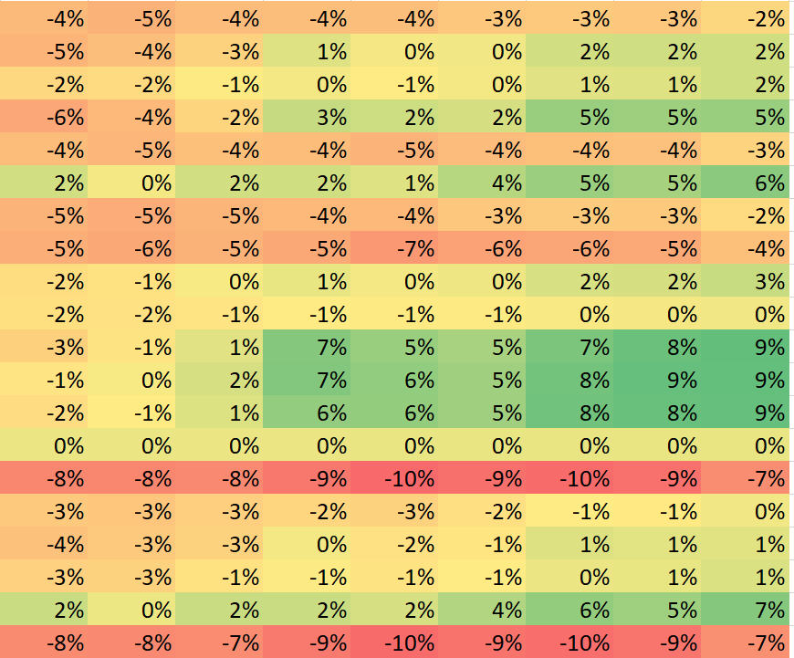
This first image is the color scale created across some of the columns together. So some columns will be missing some green colors (for max values)


h5uTj.png


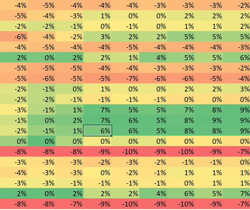
This second image is what i want, 3 color scale created in each column one by one.

Thanks.
 

Excel Facts

Format cells as time
Select range and press Ctrl+Shift+2 to format cells as time. (Shift 2 is the @ sign).
would you be opposed to using VBA?

basically, it is the same thing you described above, but instead of selecting each column yourself, you let excel select the individual columns inside those columns for you.


VBA Code:
Sub RunFormattedConditionings()

    Dim Sel As Range
    Set Sel = Selection
    
    Dim Sr As Long
    Dim Er As Long
    
    Dim Sc As Long
    Dim Ec As Long
    
    Sr = Sel.Row
    Er = Sr + Sel.Rows.Count - 1
    
    Sc = Sel.Column
    Ec = Sc + Sel.Columns.Count - 1
    
    For i = Sc To Ec
        Dim rng As Range
        Set rng = Range(Cells(Sr, i), Cells(Er, i))
        rng.FormatConditions.AddColorScale ColorScaleType:=3
        rng.FormatConditions(rng.FormatConditions.Count).SetFirstPriority
        rng.FormatConditions(1).ColorScaleCriteria(3).Type = _
            xlConditionValueHighestValue
        With rng.FormatConditions(1).ColorScaleCriteria(3).FormatColor
            .Color = 8109667
            .TintAndShade = 0
        End With
    Next


End Sub

how this code works is by selecting the range of all your data, and running the macro. Excel will loop through each column in the range you selected and change the conditional formatting to only look at one column at a time.
 
Upvote 0
I am sorry, but using a huge VBA script to solve this problem is just nuts!
To do this quickly and easily, select one entire column (A:A) and apply the conditional formatting. Then double click the Format Painter - this will lock it ON until you hit [Esc]. Now select the rest of the columns one at a time. Hit [Esc] when done. All of the columns will now have the same Conditional Formatting that was applied to column A:A but reference the correct column.
Book1
ABCDEFGHI
13%-7%1%3%5%9%-8%-4%-9%
2%6%8%9%8%%6%-5%-2%
3-6%4%-6%4%-7%-5%-3%-6%4%
4-7%-7%2%-2%9%8%-5%-1%-2%
5-3%4%5%6%%8%%-6%-5%
64%3%1%5%2%8%1%8%5%
78%9%-8%4%-1%1%-2%-8%4%
8-8%5%-4%-2%-5%5%-2%8%1%
9%4%4%2%-7%2%-6%-9%7%
10-5%9%-4%-8%-1%8%-8%6%4%
113%3%7%2%1%-3%-6%-4%6%
12-7%5%6%5%-4%1%-4%-6%-1%
136%9%-8%7%%-5%4%-3%-5%
142%-1%-8%-8%6%-8%-2%-8%-1%
159%-3%2%-5%8%-1%9%9%9%
16%2%1%6%4%-5%2%2%6%
17-8%-7%-7%-3%1%6%-7%-8%-6%
184%-5%5%-6%-8%-5%7%-1%-7%
19-7%-6%-8%3%-2%4%-9%-2%-5%
203%8%2%3%8%6%-9%-6%8%
21
22
23
Sheet1
Cell Formulas
RangeFormula
A1:I20A1=RANDARRAY(20,9,-0.09,0.09,0)
Dynamic array formulas.
Cells with Conditional Formatting
CellConditionCell FormatStop If True
I:IOther TypeColor scaleNO
H:HOther TypeColor scaleNO
G:GOther TypeColor scaleNO
F:FOther TypeColor scaleNO
E:EOther TypeColor scaleNO
D:DOther TypeColor scaleNO
C:COther TypeColor scaleNO
B:BOther TypeColor scaleNO
A:AOther TypeColor scaleNO

Note that the actual conditional formatting is done for each cell locked - "=$B:$B" not "=B:B" as indicated above, and something I didn't think would work, but the blank cells have no fill. Of course, no promises of what will show up if anything appears below the range in question. However, you can always do a fixed range in the first column like $A1:$A10000 if that becomes a problem, and then instead of selecting the entire column for the Format Painter, just select the range and then click in the first row of the range in each column:
Book1
KLMNOPQRS
1-6%-4%-5%7%8%-9%-3%-7%-7%
26%-5%-4%6%-1%%6%-3%3%
34%-9%-7%-2%-7%2%-8%1%6%
4-8%2%-5%-3%1%8%-7%2%4%
57%-3%-7%7%-1%-6%-5%%8%
6-8%3%-3%-4%1%-1%6%7%%
77%-1%3%-5%4%-5%-4%-2%-8%
8-5%-3%8%8%-6%-8%3%-4%6%
9-8%7%-6%1%-5%4%-3%-1%3%
106%-8%-6%6%-4%3%-7%1%9%
111%2%-1%-4%-1%-9%9%2%-5%
12%-7%-4%-8%-6%-2%8%-1%1%
13-4%-4%6%-3%-2%-5%2%2%-4%
14-6%3%3%-6%-2%4%9%1%-5%
157%8%8%-9%-5%-6%8%-2%2%
169%1%-3%-1%1%1%7%9%-2%
17-5%7%-1%-1%-4%2%4%9%4%
189%-6%4%4%7%-5%6%5%7%
19-7%-3%9%-6%2%6%6%8%-2%
20-9%-4%-1%-7%-4%-7%6%4%4%
21
22
23
24
25
26
27
28
29
30
Sheet1
Cell Formulas
RangeFormula
K1:S20K1=RANDARRAY(20,9,-0.09,0.09,0)
Dynamic array formulas.
Cells with Conditional Formatting
CellConditionCell FormatStop If True
S1:S29Other TypeColor scaleNO
R1:R29Other TypeColor scaleNO
Q1:Q29Other TypeColor scaleNO
P1:P29Other TypeColor scaleNO
O1:O29Other TypeColor scaleNO
N1:N29Other TypeColor scaleNO
M1:M29Other TypeColor scaleNO
L1:L29Other TypeColor scaleNO
K1:K29Other TypeColor scaleNO

Again the ranges are locked, and the cell formatting in both samples is custom #%, not blank. Also notice the conditional formatting ends at row 29 in the second sample, so putting a value of 1 in cell K24 which is included in the conditional formatting will totally screw up the colors in K1:K20. K24 will be green, and K1:K20 will all be red to yellow since they're ALL lower than 1!
 
Upvote 0
I am sorry, but using a huge VBA script to solve this problem is just nuts!
To do this quickly and easily, select one entire column (A:A) and apply the conditional formatting. Then double click the Format Painter - this will lock it ON until you hit [Esc]. Now select the rest of the columns one at a time. Hit [Esc] when done. All of the columns will now have the same Conditional Formatting that was applied to column A:A but reference the correct column.

No offense, but how was my code long, and how is your way quicker? They were trying to avoid going through and manually selecting each column individually. Am I misunderstanding?
 
Upvote 0
No offense, but how was my code long, and how is your way quicker? They were trying to avoid going through and manually selecting each column individually. Am I misunderstanding?
Well for one thing I don't have to go through hoops to save the file as an XLSM file. Also, regardless of how "safe" an Excel file might be, a Macro file is still vulnerable which is why there are so many restrictions on them. Finally, if one wants to do this on another file it would have to start with a copy of the Macro file, or the Macro would need to be copied to the new file.
I notice you don't count on any time you took to develop the script. I didn't know for sure how this would work, but it took more time to get the formatting of the numbers right than figuring out how to get the desired result. And your script requires selecting each range and then executing the script as opposed to double clicking once and then clicking on the range needed until done - a heck of a lot easier and quicker.
No offense, but you really need to ask?
 
Upvote 0
Now select the rest of the columns one at a time.
But that's exactly what the OP wanted to avoid.
And your script requires selecting each range and then executing the script as opposed to double clicking once and then clicking on the range needed until done - a heck of a lot easier and quicker.
I very much doubt that selecting each column manually & using the format painter would be quicker or easier than selecting all the columns & running one simple macro.
 
Upvote 0
Thanks for your insight.
Well for one thing I don't have to go through hoops to save the file as an XLSM file.
You can save it as an XLSM file. But, if this is a one shot thing, just delete the macro when you are done. Then you would not have to worry about it. If you do want to save it though, File> Save As> XLSM is still fewer steps than you suggested.

if one wants to do this on another file it would have to start with a copy of the Macro file, or the Macro would need to be copied to the new file.
You are saying that they would need to follow the same steps? Well... Yes? As they would with yours??

I notice you don't count on any time you took to develop the script. I didn't know for sure how this would work, but it took more time to get the formatting of the numbers right than figuring out how to get the desired result.
Yes, I have tested the script, and it works. I tested it before I posted it, as I do with all my scripts.
And yes, it did take me longer to generate random numbers than it took to format them with conditional formatting. That is precisely why VBA is useful.

Your script requires selecting each range and then executing the script as opposed to double clicking once and then clicking on the range needed until done - a heck of a lot easier and quicker.
No offense, but you really need to ask?
No, using my script you do not need to select each column. You select all the columns and the macro loops them.

It seems to me that you are simply apposed to macros. Which is fine.

It took me less than a second to preform the conditional formatting in the images provided. The clock references how long it took to change tabs to take a picture. (I would upload high quality but the Mr. Excel website would not allow full screen grabs - either case, you get the idea).

So, in short, yes, I really DO need to ask?
 

Attachments

  • save1.JPG
    save1.JPG
    208.2 KB · Views: 10
  • save2.JPG
    save2.JPG
    195.2 KB · Views: 10
Upvote 0
But that's exactly what the OP wanted to avoid.

I very much doubt that selecting each column manually & using the format painter would be quicker or easier than selecting all the columns & running one simple macro.
Errr, that has to be done with the Macro if there's more than a single range as in "Set Sel = Selection".
And you're ready to ignore all of the other issues? Fine. It ends up this question was asked again, but this time for Rows, and the user specified they didn't want to use Format Painter, and I realize that is a PITA. It ends up the solution is even easier than my previous post! Select the first column and apply the conditional formatting as needed. Now select the remaining range and select Paste -> Formatting (R) or use the Paste -> Paste Special... menu item and select Formats from the dialog box.
What's interesting about this technique is that the range the conditional formatting becomes the top left to the bottom right of the range selected, yet the formatting follows the method applied to the original row/column. This table was made using the Format Painter as explained above, manually copying the format to all 49 rows:
Book1
ABCDEFGHIJKLMNOPQRST
1308903012846976636713899194783620495156
25029115643254539842031905375799313201611
32643965050407085964928338611682433355551
4811976634055905518929354185756652143266
528337542686159486952377750428156424613
63068293431535382097683356962314221599
76856132396296236955151272886955738338
847684828152832728728536731463916409066
942631164619751767114568338773990438117100
105198812869535137327342376172694187158096
11286740562998491797479360809596929853
12459013694575533451396437884335844543221
13914932733568794710297434637934724997
148873513024394536973316510025121856231
156774944019665451119139219559283353348222
1695685134145093329371251186299122117270
17788327305195952919427307523871521950
18822011482339827779833692677677953918551
198719850367363813971375132499477612638
2057582989115762586985637036809411431052
21468222654115728587215689696785992878
22873348318761002070642552744351854309877
23854892261052195965198884475934883514197
2444326894728246591529059752228508084982
2590648157671923074720861837611049772254
263138411252811229282095808216801297169277
27538680685556196894958761972369389624636
28444777523740701399903725623956753561750
2933291849182993832990239521832737496669
30842654988816100568191229420837493121586
314288682256760919665504965402371779596
32973296100772869267225642376492637926856
334537385088774672758243428557279242457
3495536251642915690128152569592275631198
35535355665132844278233238760123950107654
3696277482604647144195849351165475383629
373465778677304142655726464526779447324045
3830449675375462804327609013678978792499
3967504426442232606019696618793147479793
40837585476279219213481875240758522659
413963128136762077174907112385125571110
4227100329192587109349982194160153508216
436152924188689527366197263521927345691
44703629611321178883236741287555755451174
4546301006749632949914639422988881244334324
4665741953786129694585864955652163786674
475478631645966747308318606871234385678573
4871921795749830284340565626314778541735
49191547953949028402846303284136769709732
5080239188845290322086943561893880836827
Sheet1
Cells with Conditional Formatting
CellConditionCell FormatStop If True
A50:T50Other TypeColor scaleNO
A49:T49Other TypeColor scaleNO
A48:T48Other TypeColor scaleNO
A47:T47Other TypeColor scaleNO
A46:T46Other TypeColor scaleNO
A45:T45Other TypeColor scaleNO
A44:T44Other TypeColor scaleNO
A43:T43Other TypeColor scaleNO
A42:T42Other TypeColor scaleNO
A41:T41Other TypeColor scaleNO
A40:T40Other TypeColor scaleNO
A39:T39Other TypeColor scaleNO
A38:T38Other TypeColor scaleNO
A37:T37Other TypeColor scaleNO
A36:T36Other TypeColor scaleNO
A35:T35Other TypeColor scaleNO
A34:T34Other TypeColor scaleNO
A33:T33Other TypeColor scaleNO
A32:T32Other TypeColor scaleNO
A31:T31Other TypeColor scaleNO
A30:T30Other TypeColor scaleNO
A29:T29Other TypeColor scaleNO
A28:T28Other TypeColor scaleNO
A27:T27Other TypeColor scaleNO
A26:T26Other TypeColor scaleNO
A25:T25Other TypeColor scaleNO
A24:T24Other TypeColor scaleNO
A23:T23Other TypeColor scaleNO
A22:T22Other TypeColor scaleNO
A21:T21Other TypeColor scaleNO
A20:T20Other TypeColor scaleNO
A19:T19Other TypeColor scaleNO
A18:T18Other TypeColor scaleNO
A17:T17Other TypeColor scaleNO
A16:T16Other TypeColor scaleNO
A15:T15Other TypeColor scaleNO
A14:T14Other TypeColor scaleNO
A13:T13Other TypeColor scaleNO
A12:T12Other TypeColor scaleNO
A11:T11Other TypeColor scaleNO
A10:T10Other TypeColor scaleNO
A9:T9Other TypeColor scaleNO
A8:T8Other TypeColor scaleNO
A7:T7Other TypeColor scaleNO
A6:T6Other TypeColor scaleNO
A5:T5Other TypeColor scaleNO
A4:T4Other TypeColor scaleNO
A3:T3Other TypeColor scaleNO
A2:T2Other TypeColor scaleNO
A1:T1Other TypeColor scaleNO

Notice that the conditional formatting is applied to each row individually.
This table was done copying the first row that had the conditional formatting, and then selecting the other 49 rows of data and using Paste -> Format:
Book1
VWXYZAAABACADAEAFAGAHAIAJAKALAMANAO
1308903012846976636713899194783620495156
25029115643254539842031905375799313201611
32643965050407085964928338611682433355551
4811976634055905518929354185756652143266
528337542686159486952377750428156424613
63068293431535382097683356962314221599
76856132396296236955151272886955738338
847684828152832728728536731463916409066
942631164619751767114568338773990438117100
105198812869535137327342376172694187158096
11286740562998491797479360809596929853
12459013694575533451396437884335844543221
13914932733568794710297434637934724997
148873513024394536973316510025121856231
156774944019665451119139219559283353348222
1695685134145093329371251186299122117270
17788327305195952919427307523871521950
18822011482339827779833692677677953918551
198719850367363813971375132499477612638
2057582989115762586985637036809411431052
21468222654115728587215689696785992878
22873348318761002070642552744351854309877
23854892261052195965198884475934883514197
2444326894728246591529059752228508084982
2590648157671923074720861837611049772254
263138411252811229282095808216801297169277
27538680685556196894958761972369389624636
28444777523740701399903725623956753561750
2933291849182993832990239521832737496669
30842654988816100568191229420837493121586
314288682256760919665504965402371779596
32973296100772869267225642376492637926856
334537385088774672758243428557279242457
3495536251642915690128152569592275631198
35535355665132844278233238760123950107654
3696277482604647144195849351165475383629
373465778677304142655726464526779447324045
3830449675375462804327609013678978792499
3967504426442232606019696618793147479793
40837585476279219213481875240758522659
413963128136762077174907112385125571110
4227100329192587109349982194160153508216
436152924188689527366197263521927345691
44703629611321178883236741287555755451174
4546301006749632949914639422988881244334324
4665741953786129694585864955652163786674
475478631645966747308318606871234385678573
4871921795749830284340565626314778541735
49191547953949028402846303284136769709732
5080239188845290322086943561893880836827
Sheet1
Cells with Conditional Formatting
CellConditionCell FormatStop If True
V2:AO50Other TypeColor scaleNO
V1:AO1Other TypeColor scaleNO

AND, as it ends up, this was all in vain. Selecting the entire range at once produces the identical results as the other two methods:
Book1
AQARASATAUAVAWAXAYAZBABBBCBDBEBFBGBHBIBJ
1308903012846976636713899194783620495156
25029115643254539842031905375799313201611
32643965050407085964928338611682433355551
4811976634055905518929354185756652143266
528337542686159486952377750428156424613
63068293431535382097683356962314221599
76856132396296236955151272886955738338
847684828152832728728536731463916409066
942631164619751767114568338773990438117100
105198812869535137327342376172694187158096
11286740562998491797479360809596929853
12459013694575533451396437884335844543221
13914932733568794710297434637934724997
148873513024394536973316510025121856231
156774944019665451119139219559283353348222
1695685134145093329371251186299122117270
17788327305195952919427307523871521950
18822011482339827779833692677677953918551
198719850367363813971375132499477612638
2057582989115762586985637036809411431052
21468222654115728587215689696785992878
22873348318761002070642552744351854309877
23854892261052195965198884475934883514197
2444326894728246591529059752228508084982
2590648157671923074720861837611049772254
263138411252811229282095808216801297169277
27538680685556196894958761972369389624636
28444777523740701399903725623956753561750
2933291849182993832990239521832737496669
30842654988816100568191229420837493121586
314288682256760919665504965402371779596
32973296100772869267225642376492637926856
334537385088774672758243428557279242457
3495536251642915690128152569592275631198
35535355665132844278233238760123950107654
3696277482604647144195849351165475383629
373465778677304142655726464526779447324045
3830449675375462804327609013678978792499
3967504426442232606019696618793147479793
40837585476279219213481875240758522659
413963128136762077174907112385125571110
4227100329192587109349982194160153508216
436152924188689527366197263521927345691
44703629611321178883236741287555755451174
4546301006749632949914639422988881244334324
4665741953786129694585864955652163786674
475478631645966747308318606871234385678573
4871921795749830284340565626314778541735
49191547953949028402846303284136769709732
5080239188845290322086943561893880836827
Sheet1
Cells with Conditional Formatting
CellConditionCell FormatStop If True
AQ1:BJ50Other TypeColor scaleNO

I'm not sure I understand why all three conditional format ranges behave the same, but they do appear to! I scanned most of the rows of all three tables, and as far as I can tell they're all the same even though the ranges that the conditional formatting is being applied to are different. I think (know?) the reason why it's working is because the color scale is based on Percentile and not the numbers themselves although percent worked as well.
 
Upvote 0
If you want to do this with rows you can change my Macro around to loop through them as well. Just replace:

VBA Code:
    For i = Sc To Ec
        Dim rng As Range
        Set rng = Range(Cells(Sr, i), Cells(Er, i))

with

VBA Code:
    For i = Sr To Er
        Dim rng As Range
        Set rng = Range(Cells(i, Sc), Cells(i, Ec))
 
Upvote 0
I am sorry, but using a huge VBA script to solve this problem is just nuts!
To do this quickly and easily, select one entire column (A:A) and apply the conditional formatting. Then double click the Format Painter - this will lock it ON until you hit [Esc]. Now select the rest of the columns one at a time. Hit [Esc] when done. All of the columns will now have the same Conditional Formatting that was applied to column A:A but reference the correct column.
Book1
ABCDEFGHI
13%-7%1%3%5%9%-8%-4%-9%
2%6%8%9%8%%6%-5%-2%
3-6%4%-6%4%-7%-5%-3%-6%4%
4-7%-7%2%-2%9%8%-5%-1%-2%
5-3%4%5%6%%8%%-6%-5%
64%3%1%5%2%8%1%8%5%
78%9%-8%4%-1%1%-2%-8%4%
8-8%5%-4%-2%-5%5%-2%8%1%
9%4%4%2%-7%2%-6%-9%7%
10-5%9%-4%-8%-1%8%-8%6%4%
113%3%7%2%1%-3%-6%-4%6%
12-7%5%6%5%-4%1%-4%-6%-1%
136%9%-8%7%%-5%4%-3%-5%
142%-1%-8%-8%6%-8%-2%-8%-1%
159%-3%2%-5%8%-1%9%9%9%
16%2%1%6%4%-5%2%2%6%
17-8%-7%-7%-3%1%6%-7%-8%-6%
184%-5%5%-6%-8%-5%7%-1%-7%
19-7%-6%-8%3%-2%4%-9%-2%-5%
203%8%2%3%8%6%-9%-6%8%
21
22
23
Sheet1
Cell Formulas
RangeFormula
A1:I20A1=RANDARRAY(20,9,-0.09,0.09,0)
Dynamic array formulas.
Cells with Conditional Formatting
CellConditionCell FormatStop If True
I:IOther TypeColor scaleNO
H:HOther TypeColor scaleNO
G:GOther TypeColor scaleNO
F:FOther TypeColor scaleNO
E:EOther TypeColor scaleNO
D:DOther TypeColor scaleNO
C:COther TypeColor scaleNO
B:BOther TypeColor scaleNO
A:AOther TypeColor scaleNO

Note that the actual conditional formatting is done for each cell locked - "=$B:$B" not "=B:B" as indicated above, and something I didn't think would work, but the blank cells have no fill. Of course, no promises of what will show up if anything appears below the range in question. However, you can always do a fixed range in the first column like $A1:$A10000 if that becomes a problem, and then instead of selecting the entire column for the Format Painter, just select the range and then click in the first row of the range in each column:
Book1
KLMNOPQRS
1-6%-4%-5%7%8%-9%-3%-7%-7%
26%-5%-4%6%-1%%6%-3%3%
34%-9%-7%-2%-7%2%-8%1%6%
4-8%2%-5%-3%1%8%-7%2%4%
57%-3%-7%7%-1%-6%-5%%8%
6-8%3%-3%-4%1%-1%6%7%%
77%-1%3%-5%4%-5%-4%-2%-8%
8-5%-3%8%8%-6%-8%3%-4%6%
9-8%7%-6%1%-5%4%-3%-1%3%
106%-8%-6%6%-4%3%-7%1%9%
111%2%-1%-4%-1%-9%9%2%-5%
12%-7%-4%-8%-6%-2%8%-1%1%
13-4%-4%6%-3%-2%-5%2%2%-4%
14-6%3%3%-6%-2%4%9%1%-5%
157%8%8%-9%-5%-6%8%-2%2%
169%1%-3%-1%1%1%7%9%-2%
17-5%7%-1%-1%-4%2%4%9%4%
189%-6%4%4%7%-5%6%5%7%
19-7%-3%9%-6%2%6%6%8%-2%
20-9%-4%-1%-7%-4%-7%6%4%4%
21
22
23
24
25
26
27
28
29
30
Sheet1
Cell Formulas
RangeFormula
K1:S20K1=RANDARRAY(20,9,-0.09,0.09,0)
Dynamic array formulas.
Cells with Conditional Formatting
CellConditionCell FormatStop If True
S1:S29Other TypeColor scaleNO
R1:R29Other TypeColor scaleNO
Q1:Q29Other TypeColor scaleNO
P1:P29Other TypeColor scaleNO
O1:O29Other TypeColor scaleNO
N1:N29Other TypeColor scaleNO
M1:M29Other TypeColor scaleNO
L1:L29Other TypeColor scaleNO
K1:K29Other TypeColor scaleNO

Again the ranges are locked, and the cell formatting in both samples is custom #%, not blank. Also notice the conditional formatting ends at row 29 in the second sample, so putting a value of 1 in cell K24 which is included in the conditional formatting will totally screw up the colors in K1:K20. K24 will be green, and K1:K20 will all be red to yellow since they're ALL lower than 1!

Thanks. I don't know if i understand completely. I tried your method and seems it doesn't work.
What I did is simply create a 3 color scale for column A, and double clicked "Format Painter", and paste across the rest of the columns in one go. The 3 color scale in the rest of the columns are still treated as an array rather than individual columns.
I am not sure if I missed some steps from text, but I don't quite understand the paragraph "Note that the actual conditional formatting is done for each cell locked - "=$B:$B" not "=B:B" as indicated above... "

For example, I have created the 3 color scale in the column A below and do format painter to column B to G in one go. As you can see, column B to G conditional formatting is still reading the data together, especially in the case if the max value in one column stand out particularly.

1680962963270.png
 
Upvote 0

Forum statistics

Threads
1,215,255
Messages
6,123,896
Members
449,132
Latest member
Rosie14

We've detected that you are using an adblocker.

We have a great community of people providing Excel help here, but the hosting costs are enormous. You can help keep this site running by allowing ads on MrExcel.com.
Allow Ads at MrExcel

Which adblocker are you using?

Disable AdBlock

Follow these easy steps to disable AdBlock

1)Click on the icon in the browser’s toolbar.
2)Click on the icon in the browser’s toolbar.
2)Click on the "Pause on this site" option.
Go back

Disable AdBlock Plus

Follow these easy steps to disable AdBlock Plus

1)Click on the icon in the browser’s toolbar.
2)Click on the toggle to disable it for "mrexcel.com".
Go back

Disable uBlock Origin

Follow these easy steps to disable uBlock Origin

1)Click on the icon in the browser’s toolbar.
2)Click on the "Power" button.
3)Click on the "Refresh" button.
Go back

Disable uBlock

Follow these easy steps to disable uBlock

1)Click on the icon in the browser’s toolbar.
2)Click on the "Power" button.
3)Click on the "Refresh" button.
Go back
Back
Top