Conditional Formatting of VLOOKUP, Newbie in need of assistance.

[BruceW123]

Hi all,

New to the forum. I am a treasurer who needs to track who owes money. As money comes in I fill in names in a speadsheet weekly, which calculates whether someone has paid their weekly fee, or owes money.
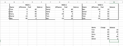
I have attached a photo of my excel sheet. I have a VLOOKUP with a column which calculates someone's overall debt. What i would, is a way to conditionally format so that said person's name in the weekly column changes colour to red if they fall below 0 in the bottom right corner where the VLOOKUP table is. Can someone help? Thanks in advance.

 

[etaf]

try
assuming the data is in Sheet1
use this and copy down
=SUM(IF(Sheet1!$B$2:$J$6=A2,Sheet1!$C$2:$K$6,0))

Book2
	A	B	C
1	Name	Charge	Balance
2	Tom	40	-70
3	Nick	40	5
4	Harry	40	-30
5	Darryl	40	0
6	Ben	30	10
Sheet2

Cell Formulas
Range	Formula
C2:C6	C2	=SUM(IF(Sheet1!$B$2:$J$6=A2,Sheet1!$C$2:$K$6,0))

 

[BruceW123]

try
assuming the data is in Sheet1
use this and copy down
=SUM(IF(Sheet1!$B$2:$J$6=A2,Sheet1!$C$2:$K$6,0))

Book2
	A	B	C
1	Name	Charge	Balance
2	Tom	40	-70
3	Nick	40	5
4	Harry	40	-30
5	Darryl	40	0
6	Ben	30	10
Sheet2

Cell Formulas
Range	Formula
C2:C6	C2	=SUM(IF(Sheet1!$B$2:$J$6=A2,Sheet1!$C$2:$K$6,0))

I've done this, i'd done it initially, but i didnt know how to do the conditional formatting we did in the first part when the table was in sheet 2. When i remove the table from sheet 1, all the coloured formatting disappears. When i try to apply your formula but change it, it doesnt work. Do you have a conditional format sequence for when the table is in sheet 2?

 

[etaf]

ok, sorry miss understood that
so you need to use

but refer to the new sheet reference
=COUNTIFS(sheet2!$A$2:$A$16,B3,sheet2!$C$2:$C$6,"<"&0) as a conditional formatting rule

 

[BruceW123]

hi,

Thank you for all your help. I set eveything up, and while it works, it seems to completely break down when i remove names or edit columns. Think it has something to do with the look up from the table. It's too delicate for me to share with other people. Thank you for your help though.

You mentioned that were better ways to set up a running balance. If you have time, could you show me a small example that i could copy and expand. What i need is to be able to add the amounts in every week but also be able to visibly see on the first sheet whether someone is in debt, hence the colours. If you know of a better way, please do let me know. Thanks again for spending the time to show me these changes.

 

[etaf]

Ok , it more to do with layout i think , but that will depend on how you want to setout the sheet
as you only showed 3 weeks

how many weeks do you go for ??
how many names may appear

so on the summary we are using

=COUNTIFS(sheet2!$A$2:$A$16,B3,sheet2!$C$2:$C$6,"<"&0)
now if more people are added the range is not big enough

how many people total are there likely to be - lets say 100 then change the range to include all possible names

=COUNTIFS(sheet2!$A$2:$A$100,B3,sheet2!$C$2:$C$100,"<"&0)

you could maybe enter names all in 1 column and dates

as you are using version 365 , you can pull across to sheet2 a set of unique names and then use that as a summary

there a few ways , but you cannot share the real data , even if desensitised at all ?

this sort of thing, summary could be on a different sheet

but i dont know enough about how you collect and record the money

Book2
	A	B	C	D	E	F	G	H	I	J	K
1				amount due	amout paid	balancve				Unique names
2	bob	1/1/23	week1	40	40	0				bob	0
3	john	1/1/23	week1	40	10	-30				john	-60
4	jill	1/1/23	week1	40	20	-20				jill	-50
5	fred	1/1/23	week1	40	40	0				fred	-40
6	susan	1/1/23	week1	40	40	0				susan	0
7	christine	1/1/23	week1	40		-40				christine	-40
8	harry	1/1/23	week1	40	40	0				harry	0
9	bob	1/7/23	week2	40	40	0
10	john	1/7/23	week2	40	10	-30
11	jill	1/7/23	week2	40	10	-30
12	fred	1/7/23	week2	40		-40
Sheet3

Cell Formulas
Range	Formula
J2:J8	J2	=UNIQUE(FILTER(A:A,A:A<>""))
F2:F12	F2	=E2-D2
K2:K12	K2	=IF(J2="","",SUMIFS($E$2:$E$100,$A$2:$A$100,J2)-SUMIFS($D$2:$D$100,$A$2:$A$100,J2))
Dynamic array formulas.