Conditional Formatting

[RobertH]

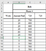
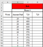
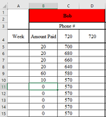
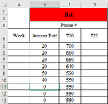
I have an Excel sheet that tracks the amount people have paid each week. I'm trying to make it so that the person's name is highlighted in red if the amount of their remaining balance is greater than it should be. I have no problem doing this portion. My problem lies with the upcoming weeks. If someone misses a payment, but the next payment drops their balance within the correct amount, the name remains red since the previous week's value has not changed. My C cell reference another cell to determine if the price is higher or lower than it should be. In the attached images, you can see when cell C9 has the correct amount, it has no color, and when C9 has the wrong amount, it changes to red. If C9 has the correct amount and C10 has the wrong amount, it will also change red, but if C9 has the wrong amount and C10 has the correct amount, it remains red even though the latest cell has the correct amount. Is there any way around this? For the formula in the conditional formatting, I was using =C9>AG9 as the formula and then =C10>AG10 as another rule, and so on.

 

[dreid1011]

What is in column AG? I assume that is the amount to determine if the balance is within the correct range. Also, out of the three images that show the name is red, which of them should NOT be red?

Or provide some sample data with the expected highlight results please.

 

[RobertH]

What is in column AG? I assume that is the amount to determine if the balance is within the correct range. Also, out of the three images that show the name is red, which of them should NOT be red?

Or provide some sample data with the expected highlight results please.

Column AG is just a reference amount to where their payments should be on that specific week. The last picture is the one that should not be red where the cell c10 is 550 since its less than the reference amount of 560.

 

[dreid1011]

Give this a try:

=INDIRECT("C"&INDEX(ROW(B5:B20),COUNTA(B5:B20)))>INDIRECT("AG"&INDEX(ROW(B5:B20),COUNTA(B5:B20)))

Make sure to change the B5:B20 range to suit your data.

 

[RobertH]

Give this a try:

=INDIRECT("C"&INDEX(ROW(B5:B20),COUNTA(B5:B20)))>INDIRECT("AG"&INDEX(ROW(B5:B20),COUNTA(B5:B20)))

Make sure to change the B5:B20 range to suit your data.

Thank you for the help so far. It's better than what I had initially; however, since I'm inputting the amounts week by week, the red won't go away until the final amount has been paid off or, in this case, all of the numbers are matching. As the weeks go by, I need them to turn red if they haven't paid for that week, but once their balance is back in good standing, the red goes away.

 

[dreid1011]

Thank you for the help so far. It's better than what I had initially; however, since I'm inputting the amounts week by week, the red won't go away until the final amount has been paid off or, in this case, all of the numbers are matching. As the weeks go by, I need them to turn red if they haven't paid for that week, but once their balance is back in good standing, the red goes away.

Okay, I am not sure I understand then. The way it is working now is if the week of the most recent payment has satisfied the comparison with col AG then the red goes away. Until then, it remains red. What other times should it remain red?

 

[RobertH]

Okay, I am not sure I understand then. The way it is working now is if the week of the most recent payment has satisfied the comparison with col AG then the red goes away. Until then, it remains red. What other times should it remain red?

My apologies. It is working correctly. It was keeping it red constantly because I had 0s as placeholders. Thanks for the help!

 

[dreid1011]

My apologies. It is working correctly. It was keeping it red constantly because I had 0s as placeholders. Thanks for the help!

Oh yes, I intended to mention that before that anything other than blanks would alter the outcome. I am glad it works, and thank you for the feedback.