conditional formatting with multiple conditions

[Kyttdina]

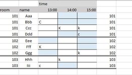
column a= room number, column B person name, column C,D, E= cells which should be highlighted after the data (K) is manually inserted
if anyone in the same room is K the others should be highlighted
If anyone from the same room is C or empty then no highlight is needed
If anyone in the room is K, then C will be entered into highlighted cell
(the highlight is necessary for not having two K at the same time in same room)

i hope i explained it well enough (English is my third language, i apologize for mistakes)
thank you in advance

 

[Kyttdina]

i will try to edit the question:
Everyone in same room (f.e 102) should be highlighted, if anyone in that room will be marked with K in column C,D,E (f.e at 13:00 person Fff in room 102 is marked K, so persons Eee and Ggg should be highlighted) If anyone from the same room is marked C or empty in columns C,D, E then no highlight. If there is already K and the cells are highlighted, then C will be entered into highlighted cell.
i cannot figure out the formula. hopefully this explains better my struggle...

 

[Eric W]

Welcome to the forum!

Perhaps:

Book2
	A	B	C	D	E	F
1			time
2	room	name	13:00	14:00	15:00
3	101	aaa				101
4	101	bbb	C			101
5	101	ccc		K	K	101
6	101	ddd			C	101
7	102	eee				102
8	102	fff	K			102
9	102	ggg			K	102
10	103	hhh		K		103
11	103	iii	C			103
Sheet4

Cells with Conditional Formatting
Cell	Condition		Cell Format	Stop If True
B3:B11	Expression	=SUMPRODUCT(($C$3:$E$11="K")*($A$3:$A$11=A3))*(COUNTIF(C3:E3,"C")=0)	text	NO

 

[Kyttdina]

=SUMPRODUCT(($C$3:$E$11="K")*($A$3:$A$11=A3))*(COUNTIF(C3:E3,"C")=0)

i suppose i was not very clear with my explanation. i will try again:
i have for people in room 101: aaa, bbb, ccc, ddd are the names of those people.
When i give one person a task K at 13:00 i need other three people to have a highlighted cell at 13:00 so i will not accidentally give any of them the same task (K).
but thanks for your suggestion

 

[Kyttdina]

Welcome to the forum!

Perhaps:

Book2
	A	B	C	D	E	F
1			time
2	room	name	13:00	14:00	15:00
3	101	aaa				101
4	101	bbb	C			101
5	101	ccc		K	K	101
6	101	ddd			C	101
7	102	eee				102
8	102	fff	K			102
9	102	ggg			K	102
10	103	hhh		K		103
11	103	iii	C			103
Sheet4

Cells with Conditional Formatting
Cell	Condition		Cell Format	Stop If True
B3:B11	Expression	=SUMPRODUCT(($C$3:$E$11="K")*($A$3:$A$11=A3))*(COUNTIF(C3:E3,"C")=0)	text	NO

hi Eric
i used your formula and changed it a bit and now it does exactly what i need. i am so thankful to you.
i just changed it to this:
=SUMPRODUCT((C$3:C$11="K")*($A$3:$A$11=$A3))

i am so grateful!

 

[Eric W]

Glad you got it worked out! Thanks for the update!

 

[Kyttdina]

Glad you got it worked out! Thanks for the update!

could you help me once more with the same table (adding new rule)?

 

[Eric W]

What's your new rule?

 

[Kyttdina]

What's your new rule?

 

[Kyttdina]

so what i mean is:
if C2= K and ColumnA= 101 then it returns the formats in all the cells in Column C ( or any column) that have 101 in ColumnA. - that is waht it does.
what i cannot make it to do: i need same formating in Column D (or any column) if C2=K is followed by D2=2.