Conditional Formatting

[AYSHANA]

Dear all,

Good Day!

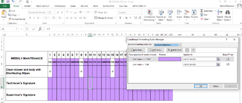
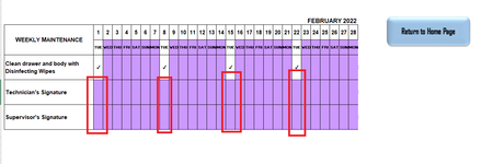
can somebody help me in the condition formatting.

I'm trying to return to the circled cells (check the attached pic) into white color, if i will select the (tick) symbol.


I'm doing maintenance every Tuesday so if ill select the tick mark for Tuesday I want to return in to white color or blank so ill be able to write my initial and supervisor sign.

NOTE: THERE IS FORMULA IN ALL THE CELLS (EXAMPLE C7=C6)(C8=C7)


if anyone have an idea how to solve it , I really appreciate .

please check the following attachment.

thank you.

 

[etaf]

you could test to see if a Tick Exists
Not sure what you are using as a tick.
I used Marlett font , lower case a = tick

and then used a formula
=C$2="a"
and filled white

Book9
	A	B	C	D	E	F	G	H	I	J	K
1
2			a			a			a
3
4
5
6
7
8
9
10
11
12
13
14
15
16
17
18
19
Sheet2

Cells with Conditional Formatting
Cell	Condition		Cell Format	Stop If True
C3:C18,F3:F18,I3:I18	Expression	=C$2="a"	text	NO

 

[AYSHANA]

im using a symbol for the tick mark, and i did it as drop list

 

[etaf]

ok, you could use the character code for the symbol in conditional formatting
not sure what symbol you have used - BUT to find the value use
=CODE(cell with the tick in)
that will give you the char() value
so you could use that as conditional formatting

so in my example above where i have =C$2="a"
then use
=C$2=char( the value from CODE(cell with the tick in))
OR you could refer the the cell that you have the symbol in for the dropdown
lets say the drop down list is in a different sheet and cell A3
then
=C$2=Sheet2!$A$3

otherwise post the spreadsheet here using XL2BB or put onto a share like dropbox/onedrive, the only shares i use

 

[Alex Blakenburg]

See if you think something like this might work for you.

Book1
	A	B	C	D
1	Symbol	UniCode	UniCode Formula
2	✓	10003	=UNICODE(A2)
3	✓
4
Sheet1

Cell Formulas
Range	Formula
B2	B2	=UNICODE(A2)
C2	C2	=FORMULATEXT(B2)

Cells with Conditional Formatting
Cell	Condition		Cell Format	Stop If True
A2:A4	Expression	=UNICODE(A2)=10003	text	NO

 

[etaf]

Book2
	B	C	D	E	F	G	H	I	J	K	L	M	N	O
1
2		✓			✓			✓				Symbol	UniCode	UniCode Formula
3												✓	10003	=UNICODE(M3)
4												✓
5
6
7
8
9
10
11
12
13
14
15
16
17
18
19
Sheet3

Cell Formulas
Range	Formula
C2	C2	=M3
F2	F2	=M3
I2	I2	=M3
N3	N3	=UNICODE(M3)
O3	O3	=FORMULATEXT(N3)

Cells with Conditional Formatting
Cell	Condition		Cell Format	Stop If True
C2:J18	Expression	=C$2=$M$3	text	NO

 

[AYSHANA]

condition

please check the link

thank you

 

[etaf]

where you have
$AK$7
change the formula in conditional formatting to be
=C$7 = $AK$7
and change the range applies to so its AD9 NOT AD7

edit
not showing here - but it does change to white
see link, i only maintain the link for a few days

Dropbox - File Deleted - Simplify your life

www.dropbox.com

condition .xlsx
	A	B	C	D	E	F	G	H	I	J	K	L	M	N	O	P	Q	R	S	T	U	V	W	X	Y	Z	AA	AB	AC	AD				AH	AI	AJ	AK
1
2
3		RESUS BLOOD BANK FRIDGE (SANYO) Maintenance
4																									FEBRUARY 2022
5		WEEKLY MAINTENANCE	1	2	3	4	5	6	7	8	9	10	11	12	13	14	15	16	17	18	19	20	21	22	23	24	25	26	27	28							TRUE
6			TUE	WED	THU	FRI	SAT	SUN	MON	TUE	WED	THU	FRI	SAT	SUN	MON	TUE	WED	THU	FRI	SAT	SUN	MON	TUE	WED	THU	FRI	SAT	SUN	MON
7		Clean drawer and body with Disinfecting Wipes	✓	WED	THU	FRI	SAT	SUN	MON	✓	WED	THU	FRI	SAT	SUN	MON	✓	WED	THU	FRI	SAT	SUN	MON	TUE	WED	THU	FRI	SAT	SUN	MON							✓
8		Technician's Signature	✓	WED	THU	FRI	SAT	SUN	MON	✓	WED	THU	FRI	SAT	SUN	MON	✓	WED	THU	FRI	SAT	SUN	MON	TUE	WED	THU	FRI	SAT	SUN	MON							✕
9		Supervisor's Signature	✓	WED	THU	FRI	SAT	SUN	MON	✓	WED	THU	FRI	SAT	SUN	MON	✓	WED	THU	FRI	SAT	SUN	MON	TUE	WED	THU	FRI	SAT	SUN	MON					note: im doing maintenace every TUE
10																																			so whenever I will select the tick mark on tue, I want to return example: cell (c8) and (c9) as blank so ill be able to sign
18
19		Reviewed by:
20			Blood Bank Incharge
21
22		Date:
BloodFridgeSanyoMTS

Cell Formulas
Range	Formula
AK5	AK5	=C7=AK7
D7:I7,C8:AD9,R7:AD7,K7:P7	D7	=D6

Cells with Conditional Formatting
Cell	Condition		Cell Format	Stop If True
C7:AD9	Expression	=C$7=$AK$7	text	YES
C6:AG6	Cell Value	="TUE"	text	YES
C6:AG6	Cell Value	<>"TUE"	text	YES
C7:AG9	Cell Value	<>"TUE"	text	YES
C7:AG9	Cell Value	="TUE"	text	YES

Cells with Data Validation
Cell	Allow	Criteria
C7:AD7	List	=$AK$7

 

[AYSHANA]

got it ,

thank you

 

[etaf]

you are welcome, glad its now resolved