Conditionally formatting doughnut chart based on non-percentage value

[Pi_Lover]

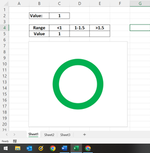
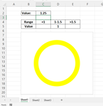
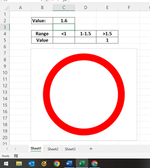
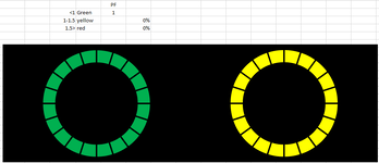
How do I conditionally format a doughnut chart based on a value that is not a percentage? Chart will remain at 100%, but I want the color to change based on a specific number value. Such as <=1 is green, >1 and <=1.5 is yellow, and >1.5 is red. Is this possible to do?

 

[kevin9999]

I think it would require a secondary table to return the % of the different ranges. So if you had an arrangement like this:

Book1
	A	B	C	D
1	Values		Range	Percent
2	2		<=1	25%
3	0.75		1-1.5	25%
4	1		>1.5	50%
5	1.25
6	1.5
7	2
8	2
9	2
Sheet1

Cell Formulas
Range	Formula
D2	D2	=COUNTIF($A$2:$A$9,"<=1")/COUNTA($A$2:$A$9)
D3	D3	=COUNTIFS($A$2:$A$9,">1",$A$2:$A$9,"<=1.5")/COUNTA($A$2:$A$9)
D4	D4	=COUNTIF($A$2:$A$9,">1.5")/COUNTA($A$2:$A$9)

You could produce a donut chart like this:

 

[Pi_Lover]

I think it would require a secondary table to return the % of the different ranges. So if you had an arrangement like this:

Book1
	A	B	C	D
1	Values		Range	Percent
2	2		<=1	25%
3	0.75		1-1.5	25%
4	1		>1.5	50%
5	1.25
6	1.5
7	2
8	2
9	2
Sheet1

Cell Formulas
Range	Formula
D2	D2	=COUNTIF($A$2:$A$9,"<=1")/COUNTA($A$2:$A$9)
D3	D3	=COUNTIFS($A$2:$A$9,">1",$A$2:$A$9,"<=1.5")/COUNTA($A$2:$A$9)
D4	D4	=COUNTIF($A$2:$A$9,">1.5")/COUNTA($A$2:$A$9)

You could produce a donut chart like this:
View attachment 102173

I wan the chart to stay at 100% permanently, but change colors depending on a value other than a percentage. If that makes sense. Meaning the entire chart reads 100" green, or yellow, or red

 

[kevin9999]

Understood. The closest I can come is by creating a table that returns either 1 or "" depending on the value of another cell. You can then overlap the three data series separately on the same chart (enabling you to format them individually) so you end up with something like this:
Data series:

Book1
	A	B	C	D	E
1
2		Value:	1.6
3
4		Range	<1	1-1.5	>1.5
5		Value			1
Sheet1

Cell Formulas
Range	Formula
C5	C5	=IF(C2<=1,1,"")
D5	D5	=IF(AND(C2>1,C2<=1.5),1,"")
E5	E5	=IF(C2>1.5,1,"")

Chart results:

 

[Pi_Lover]

Understood. The closest I can come is by creating a table that returns either 1 or "" depending on the value of another cell. You can then overlap the three data series separately on the same chart (enabling you to format them individually) so you end up with something like this:
Data series:

Book1
	A	B	C	D	E
1
2		Value:	1.6
3
4		Range	<1	1-1.5	>1.5
5		Value			1
Sheet1

Cell Formulas
Range	Formula
C5	C5	=IF(C2<=1,1,"")
D5	D5	=IF(AND(C2>1,C2<=1.5),1,"")
E5	E5	=IF(C2>1.5,1,"")

Chart results:

This works perfectly. Until I change the chart to a segmented doughnut chart. Any idea on why each color remains at 100% despite the cell value, after doing so? I've tried a few things to no avail

 

[kevin9999]

Any idea on why each color remains at 100%

Because I thought that was what you wanted:

I wan the chart to stay at 100% permanently

If you're looking for something else, I think you need to explain a bit more about your logic. A sample of both the table, and your expected outcome would be ideal.

 

[Pi_Lover]

Because I thought that was what you wanted:

If you're looking for something else, I think you need to explain a bit more about your logic. A sample of both the table, and your expected outcome would be ideal.

What I am looking for is 1 segmented doughnut chart that will change colors depending on a cell value. The overlaying of each chart works, except for when I turn it into a segmented doughnut chart. Meaning, before I change it to a segmented chart, the doughnut chart (red chart) will drop to zero % when the value changes, thus showing the next color under it. But once I change the doughnut chart to a segmented doughnut chart the each color stays at 100% and will not drop to 0% with the value change. So I can set up a standard doughnut chart and overlay all 3 over one another and the correct color goes to 100% with the value change, but not when i change the chart to a segmented doughnut chart.

 

[Pi_Lover]

I can go into more detail with the table and charts once I get home this evening. That may be more helpful

 

[kevin9999]

By "segmented doughnut chart" do you mean like what I offered in post #2? Unfortunately, my reading of your requirements is a combination of the solution in post #4 & post #2 - and I don't know how to do that. As I said, an actual sample of what you mean would be much more useful than a description.

 

[Pi_Lover]

Here is a segmented doughnut chat. Once I make the doughnut segmented, it stays 100% permanently. Even if the value changes