Consolidating 2 columns based on value in another column to another Worksheet

[goby]

I'm using the FILTER function to auto populate information from a primary Worksheet into specified columns of a secondary Worksheet. For reasons that I will leave unspecified, the primary Worksheet requires for each "Type" to have its own line item and be in different columns. Even if it is the same "Customer," "Sales Associate," or transaction in general.

I will pay my "Sales Associates" based on the amount of cake and ice cream they sell. I'd like to itemize their pay sheet but I want to consolidate "Ice Cream Type" and "Cake Type" to one column and maintain their individual rows.

I have attached some examples:
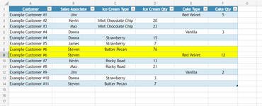
table1: Primary Worksheet (Job List)
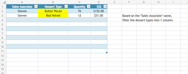
table2: Secondary Worksheet (Sales Associate Pay Sheet)


Thanks!!

 

[Kerryx]

power query

Book1
	A	B	C	D	E	F	G	H	I	J
1	Customer	Sales person	Ice Cream Type	Ice Cream Qty	Cake Type	Cake Qty		Sales person	Dessert Type	Quantity
2	#1	Jim			Red Velvet	5		Jim	Red Velvet	5
3	#2	Kevin	Mint	20				Kevin	Mint	20
4	#3	Max	Mint	23				Max	Mint	23
5	#4	Donna			Vanilla	3		Donna	Vanilla	3
6	#4	Donna	Strawberry	15				Donna	Strawberry	18
7	#5	James	Strawberry	7				James	Strawberry	7
8	#6	Steven	Pecan	76				Steven	Pecan	83
9	#6	Steven			Red Velvet	12		Steven	Red Velvet	12
10	#7	Kevin	Rocky	13				Kevin	Rocky	13
11	#8	Max	Rocky	21				Max	Rocky	21
12	#9	Jim			Vanilla	2		Jim	Vanilla	2
13	#10	Donna	Strawberry	3
14	#11	Steven	Pecan	7
Sheet1

Now someonw else may be able to provide a tidier piece of code but here is mine

let
    Source = Excel.CurrentWorkbook(){[Name="Table1"]}[Content],
    #"Changed Type" = Table.TransformColumnTypes(Source,{{"Customer", type text}, {"Sales person", type text}, {"Ice Cream Type", type text}, {"Ice Cream Qty", Int64.Type}, {"Cake Type", type text}, {"Cake Qty", Int64.Type}}),
    #"Removed Columns" = Table.RemoveColumns(#"Changed Type",{"Customer"}),
    #"Unpivoted Columns" = Table.UnpivotOtherColumns(#"Removed Columns", {"Sales person", "Ice Cream Qty", "Cake Qty"}, "Type", "Dessert Type"),
    #"Inserted Addition" = Table.AddColumn(#"Unpivoted Columns", "Quantity", each List.Sum({[Ice Cream Qty] , [Cake Qty]}), Int64.Type),
    #"Removed Columns1" = Table.RemoveColumns(#"Inserted Addition",{"Ice Cream Qty", "Cake Qty", "Type"}),
    #"Grouped Rows" = Table.Group(#"Removed Columns1", {"Sales person", "Dessert Type"}, {{"Quantity", each List.Sum([Quantity]), type number}})
in
    #"Grouped Rows"

 

[Peter_SSs]

I suggest that you investigate XL2BB for providing sample data to make it easier for helpers by not having to manually type out sample data to test with.

Not exactly sure what you are after and cannot see where $152 or $51 in the results came from, but could this be any use?

goby.xlsm
	A	B	C	D	E	F
1	Customer	Sales person	Ice Cream Type	Ice Cream Qty	Cake Type	Cake Qty
2	#1	Jim			Red Velvet	5
3	#2	Kevin	Mint Chocolate Chip	20
4	#3	Max	Mint Chocolate Chip	23
5	#4	Donna			Vanilla	3
6	#4	Donna	Strawberry	15
7	#5	James	Strawberry	7
8	#6	Steven	Butter Pecan	76
9	#6	Steven			Red Velvet	12
10	#7	Kevin	Rocky Road	13
11	#8	Max	Rocky Road	21
12	#9	Jim			Vanilla	2
13	#10	Donna	Strawberry	3
14	#11	Steven	Butter Pecan	7
Primary

goby.xlsm
	A	B	C	D
1	Sales Associate	Dessert Type	Quantity	$$$
2	Jim	Red Velvet	5
3	Kevin	Mint Chocolate Chip	20
4	Max	Mint Chocolate Chip	23
5	Donna	Vanilla	3
6	Donna	Strawberry	15
7	James	Strawberry	7
8	Steven	Butter Pecan	76
9	Steven	Red Velvet	12
10	Kevin	Rocky Road	13
11	Max	Rocky Road	21
12	Jim	Vanilla	2
13	Donna	Strawberry	3
14	Steven	Butter Pecan	7
Secondary

Cell Formulas
Range	Formula
A2:C14	A2	=HSTACK(Table1[Sales person],Table1[Ice Cream Type]&Table1[Cake Type],Table1[Ice Cream Qty]+Table1[Cake Qty])
Dynamic array formulas.

 

[goby]

power query

Book1
	A	B	C	D	E	F	G	H	I	J
1	Customer	Sales person	Ice Cream Type	Ice Cream Qty	Cake Type	Cake Qty		Sales person	Dessert Type	Quantity
2	#1	Jim			Red Velvet	5		Jim	Red Velvet	5
3	#2	Kevin	Mint	20				Kevin	Mint	20
4	#3	Max	Mint	23				Max	Mint	23
5	#4	Donna			Vanilla	3		Donna	Vanilla	3
6	#4	Donna	Strawberry	15				Donna	Strawberry	18
7	#5	James	Strawberry	7				James	Strawberry	7
8	#6	Steven	Pecan	76				Steven	Pecan	83
9	#6	Steven			Red Velvet	12		Steven	Red Velvet	12
10	#7	Kevin	Rocky	13				Kevin	Rocky	13
11	#8	Max	Rocky	21				Max	Rocky	21
12	#9	Jim			Vanilla	2		Jim	Vanilla	2
13	#10	Donna	Strawberry	3
14	#11	Steven	Pecan	7
Sheet1

Now someonw else may be able to provide a tidier piece of code but here is mine

let
    Source = Excel.CurrentWorkbook(){[Name="Table1"]}[Content],
    #"Changed Type" = Table.TransformColumnTypes(Source,{{"Customer", type text}, {"Sales person", type text}, {"Ice Cream Type", type text}, {"Ice Cream Qty", Int64.Type}, {"Cake Type", type text}, {"Cake Qty", Int64.Type}}),
    #"Removed Columns" = Table.RemoveColumns(#"Changed Type",{"Customer"}),
    #"Unpivoted Columns" = Table.UnpivotOtherColumns(#"Removed Columns", {"Sales person", "Ice Cream Qty", "Cake Qty"}, "Type", "Dessert Type"),
    #"Inserted Addition" = Table.AddColumn(#"Unpivoted Columns", "Quantity", each List.Sum({[Ice Cream Qty] , [Cake Qty]}), Int64.Type),
    #"Removed Columns1" = Table.RemoveColumns(#"Inserted Addition",{"Ice Cream Qty", "Cake Qty", "Type"}),
    #"Grouped Rows" = Table.Group(#"Removed Columns1", {"Sales person", "Dessert Type"}, {{"Quantity", each List.Sum([Quantity]), type number}})
in
    #"Grouped Rows"

Thank you very much for taking the time and for the quick response @Kerryx. I should have clarified in my original post that I not looking for power query for this solution.

 

[goby]

I suggest that you investigate XL2BB for providing sample data to make it easier for helpers by not having to manually type out sample data to test with.

Not exactly sure what you are after and cannot see where $152 or $51 in the results came from, but could this be any use?

goby.xlsm
	A	B	C	D	E	F
1	Customer	Sales person	Ice Cream Type	Ice Cream Qty	Cake Type	Cake Qty
2	#1	Jim			Red Velvet	5
3	#2	Kevin	Mint Chocolate Chip	20
4	#3	Max	Mint Chocolate Chip	23
5	#4	Donna			Vanilla	3
6	#4	Donna	Strawberry	15
7	#5	James	Strawberry	7
8	#6	Steven	Butter Pecan	76
9	#6	Steven			Red Velvet	12
10	#7	Kevin	Rocky Road	13
11	#8	Max	Rocky Road	21
12	#9	Jim			Vanilla	2
13	#10	Donna	Strawberry	3
14	#11	Steven	Butter Pecan	7
Primary

goby.xlsm
	A	B	C	D
1	Sales Associate	Dessert Type	Quantity	$$$
2	Jim	Red Velvet	5
3	Kevin	Mint Chocolate Chip	20
4	Max	Mint Chocolate Chip	23
5	Donna	Vanilla	3
6	Donna	Strawberry	15
7	James	Strawberry	7
8	Steven	Butter Pecan	76
9	Steven	Red Velvet	12
10	Kevin	Rocky Road	13
11	Max	Rocky Road	21
12	Jim	Vanilla	2
13	Donna	Strawberry	3
14	Steven	Butter Pecan	7
Secondary

Cell Formulas
Range	Formula
A2:C14	A2	=HSTACK(Table1[Sales person],Table1[Ice Cream Type]&Table1[Cake Type],Table1[Ice Cream Qty]+Table1[Cake Qty])
Dynamic array formulas.

This is more what I am looking for. First, thank you for the suggestion, I will check that out for future reference.

I'd like to say: IF "Sales Person" is "Donna", THEN HSTACK. Is this possible?

 

[Peter_SSs]

I'd like to say: IF "Sales Person" is "Donna", THEN HSTACK. Is this possible?

goby.xlsm
	A	B	C	D	E	F
1	Sales Associate	Dessert Type	Quantity	$$$		Sales Associate
2	Donna	Vanilla	3			Donna
3	Donna	Strawberry	15
4	Donna	Strawberry	3
5
Secondary

Cell Formulas
Range	Formula
A2:C4	A2	=LET(f,HSTACK(Table1[Sales person],Table1[Ice Cream Type]&Table1[Cake Type],Table1[Ice Cream Qty]+Table1[Cake Qty]),FILTER(f,TAKE(f,,1)=F2))
Dynamic array formulas.