Count Cells containing x but only under Column Heading "Contractor"

[yipppppppy]

Hi all,

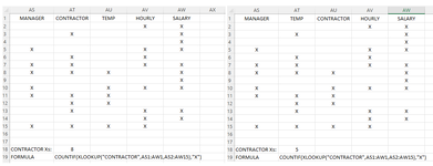
The following formula works where it counts the number of cells containing x under column where the heading is Contractor. This column is in Column AO as per formula below but how can i modify the formula below so if someone moves the Contractor Column from Column AO to another column, the formula still works?

=IFERROR(COUNTIF('CL7'!AO:AO,"x"),"Error")

 

[kevin9999]

Try this. Just change the 1000 to as many rows as you think you'll need to capture all the data.

=IFERROR(SUMPRODUCT(--('CL7'!A1:AO1="Contractor")*('CL7'!A2:AO1000="x")),"Error")

 

[yipppppppy]

Try this. Just change the 1000 to as many rows as you think you'll need to capture all the data.

=IFERROR(SUMPRODUCT(--('CL7'!A1:AO1="Contractor")*('CL7'!A2:AO1000="x")),"Error")

Thanks alot. How can i add to this formula so it only counts the above AND if the cell under "Management" Column contains "Consultant"

 

[yipppppppy]

Thanks alot. How can i add to this formula so it only counts the above AND if the cell under "Management" Column contains "Consultant"

Just to clarify, the cell under "Management" column containing the word "Consultant" it is the corresponding cell to it.

 

[RICH937]

I would approach this a little different. the formula I would use is: =IFERROR(COUNTIF(XLOOKUP("CONTRACTOR",AS1:AW1,AS2:AW15),"X"),"ERROR"). If the column containing consultant data is shifted, this will adjust the value accordingly. screenshot of swapping "contractor" and "temp" attached. if you want to select the entire columns for your range, =IFERROR(COUNTIF(XLOOKUP("CONTRACTOR",AS1:AW1,AS:AW),"X"),"ERROR") will work as well. If you're using a dynamic array with hard entered column numbers, you can use: =IFERROR(COUNTIF(XLOOKUP("CONTRACTOR",AS1:AW1,AS2#),"X"),"ERROR").

 

[yipppppppy]

 

[yipppppppy]

Hi hope the above two images help. I just need the formula for where the 74 is being returned to be actually 1 since that is the right answer.

 

[RICH937]

That won't work. "And" (*) isn't the same as "Contains." If I did the math right, you have 69 "X's" filtered in C1. There's a strong video on this on YouTube if you want to go this route. Having said that, I think that's still overly complicated. It's much easier to use Index+Filter and then CountA.
Formula: =COUNTA(FILTER(INDEX(A2:D4,,3),(A2:A4="7-MANAGER")*(B2:B4="RED")))
Result: 1
You can also use A:A and B:B. It just grows the spreadsheet unnecessarily.

 

[yipppppppy]

Hi sorry about this. Hope i make sense below.

What I am after is to add an extra condition to the below formula. It returns the correct number of x in the FY23 TP column (which is 3 by the way) so that part is fine.

All i am after now is what do i need to add to the below formula so it calculates only those that meet the above criteria AND
1) Where the corresponding column which is titled "Management Level" contains the word "Manager" AND
2) The second corresponding column which is titled "Portfolio" contains the word "Red" or "Blue"

=IFERROR(SUMPRODUCT(--('CL7'!A1:AO1="FY23 TP")*('CL7'!A2:AO100000="x")),"Error")

So if for example one of the three rows that contains x under the FY23 TP column does not have either the word Manager under Management Level, or Red or Blue under Portfolio then it should return a value less than 3.

 

[Alex Blakenburg]

You are mixing and matching in your examples in terms of what columns you are using and what criteria.
It just means you will need to do more at your end to modify anything we come up with.

See if this does what you are trying to do. You will need to modify the column and row range to accomodate your data.

20230603 CountIfs multiple criteria and Col select yipppppppy.xlsx
	A	B
1
2
3	Result	1
4
5
6	Parameterised
7	Management Level	7-Manager
8	Portfolio	Red
9	FY23 TP	X
10
11	Result	1
Result

Cell Formulas
Range	Formula
B3	B3	=COUNTIFS( INDEX('CL7'!$A$1:$AO$10000,0,MATCH("Management Level",'CL7'!$A$1:$AO$1,0)),"7-Manager", INDEX('CL7'!$A$1:$AO$10000,0,MATCH("Portfolio",'CL7'!$A$1:$AO$1,0)),"Red", INDEX('CL7'!$A$1:$AO$10000,0,MATCH("FY23 TP",'CL7'!$A$1:$AO$1,0)),"X")
B11	B11	=COUNTIFS( INDEX('CL7'!$A$1:$AO$10000,0,MATCH("Management Level",'CL7'!$A$1:$AO$1,0)),$B$7, INDEX('CL7'!$A$1:$AO$10000,0,MATCH("Portfolio",'CL7'!$A$1:$AO$1,0)),$B$8, INDEX('CL7'!$A$1:$AO$10000,0,MATCH("FY23 TP",'CL7'!$A$1:$AO$1,0)),$B$9)