Count Cells containing x but only under Column Heading "Contractor"

[yipppppppy]

Hi all,

The following formula works where it counts the number of cells containing x under column where the heading is Contractor. This column is in Column AO as per formula below but how can i modify the formula below so if someone moves the Contractor Column from Column AO to another column, the formula still works?

=IFERROR(COUNTIF('CL7'!AO:AO,"x"),"Error")

 

[Alex Blakenburg]

PS: If you could also please update your profile to show which version of excel you are using, since the solution can vary based on the version. eg you have not mentioned whether the Filter and Xlooup formulas in some of the above solutions are actually available to you.

 

[RICH937]

You are mixing and matching in your examples in terms of what columns you are using and what criteria.
It just means you will need to do more at your end to modify anything we come up with.

See if this does what you are trying to do. You will need to modify the column and row range to accomodate your data.

20230603 CountIfs multiple criteria and Col select yipppppppy.xlsx
	A	B
1
2
3	Result	1
4
5
6	Parameterised
7	Management Level	7-Manager
8	Portfolio	Red
9	FY23 TP	X
10
11	Result	1
Result

Cell Formulas
Range	Formula
B3	B3	=COUNTIFS( INDEX('CL7'!$A$1:$AO$10000,0,MATCH("Management Level",'CL7'!$A$1:$AO$1,0)),"7-Manager", INDEX('CL7'!$A$1:$AO$10000,0,MATCH("Portfolio",'CL7'!$A$1:$AO$1,0)),"Red", INDEX('CL7'!$A$1:$AO$10000,0,MATCH("FY23 TP",'CL7'!$A$1:$AO$1,0)),"X")
B11	B11	=COUNTIFS( INDEX('CL7'!$A$1:$AO$10000,0,MATCH("Management Level",'CL7'!$A$1:$AO$1,0)),$B$7, INDEX('CL7'!$A$1:$AO$10000,0,MATCH("Portfolio",'CL7'!$A$1:$AO$1,0)),$B$8, INDEX('CL7'!$A$1:$AO$10000,0,MATCH("FY23 TP",'CL7'!$A$1:$AO$1,0)),$B$9)

PS: If you could also please update your profile to show which version of excel you are using, since the solution can vary based on the version. eg you have not mentioned whether the Filter and Xlooup formulas in some of the above solutions are actually available to you.
DOH! I meant to ask that in my last post!

 

[RICH937]

Here you go. Must have: (1) X value in FY 23TP, (2) 7-Manager in Management level, (3) either Red or Blue in Portfolio.
=SUMPRODUCT(--IF(OR(B2:B4="red",B2:B4="blue"),FILTER((A1:D1="fy 23 tp")*(A2:D4="x"),A2:A4="7-manager")))

 

[yipppppppy]

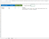
Hi all, thanks for all your help. I updated the version in my profile. I use Office 365. Unfortunately the above still doesn't work. It gives me N/A. I have posted both screenshots. The second screenshot further below is the table where the data is. Note: It is in a DIFFERENT tab to the first screenshot, the second screenshot tab is called "CL7"

Now the first tab which is the first screenshot directly below is where all my formulas are. Now where you can see 3 under column E that is derived from the formula shown in this same screenshot and copied here also. This gives the right answer of 3 as you can see there are 3 x's in the second screenshot. All i am after though is what do i need to update in this formula so it gives me the answer where:

1) There is an x under FY23 in the CL7 tab AND
2) The corresponding cell in the Management Level Column in the CL7 tab is 7-Manager AND
3) The corresponding cell in the Portfolio Column in the CL7 tab is Red or Blue

As per my second screenshot, if you work it out manually the answer is 2, but how can i update the formula below so it shows 2.

=IFERROR(SUMPRODUCT(--('CL7'!A1:AO1="FY23 TP")*('CL7'!A2:AO100000="x")),"Error")

 

[Alex Blakenburg]

Did you try my post #10 ?

 

[RICH937]

Either of these should work. I did both on a different sheet, and then copied and pasted to "CL7." I did a double check with the full columns just in case the filtered values may be throwing it off. Try pasting that formula directly into your spreadsheet. If it doesn't work....I'm stumped.
full column formula: =SUMPRODUCT(--IF(OR('CL7'!B:B="red",'CL7'!B:B="blue"),FILTER(('CL7'!A1:D1="fy 23 tp")*('CL7'!A:D="x"),'CL7'!A:A="7-manager")))
tighter formula: =SUMPRODUCT(--IF(OR('CL7'!B2:B4="red",'CL7'!B2:B4="blue"),FILTER(('CL7'!A1:D1="fy 23 tp")*('CL7'!A2:D4="x"),'CL7'!A2:A4="7-manager")))

 

[yipppppppy]

Again really appreciate your assistance here. I think i will just calculate the totals manually for now. Unless there is a feature here where i can send my spreadsheet so you can see for yourself the issue?

 

[RICH937]

Again really appreciate your assistance here. I think i will just calculate the totals manually for now. Unless there is a feature here where i can send my spreadsheet so you can see for yourself the issue?

you can throw it into a folder on the google drive, and share the link. Make sure you change permission to "editor", and share the folder not the file. The file will only open as a google sheet, which probably won't work.

 

[Alex Blakenburg]

Try

=SUM(
     (INDEX('CL7'!$A$1:$AO$10000,0,MATCH("Management Level",'CL7'!$A$1:$AO$1,0)) = "7-Manager") *
     (INDEX('CL7'!$A$1:$AO$10000,0,MATCH("Portfolio",'CL7'!$A$1:$AO$1,0)) = {"Red","Blue"}) *
     (INDEX('CL7'!$A$1:$AO$10000,0,MATCH("FY23 TP",'CL7'!$A$1:$AO$1,0)) = "X"))

 

[yipppppppy]

Try

=SUM(
     (INDEX('CL7'!$A$1:$AO$10000,0,MATCH("Management Level",'CL7'!$A$1:$AO$1,0)) = "7-Manager") *
     (INDEX('CL7'!$A$1:$AO$10000,0,MATCH("Portfolio",'CL7'!$A$1:$AO$1,0)) = {"Red","Blue"}) *
     (INDEX('CL7'!$A$1:$AO$10000,0,MATCH("FY23 TP",'CL7'!$A$1:$AO$1,0)) = "X"))