COUNTIFS up to a certain number of occurences

danthesuperman

New Member
Joined
May 25, 2020
Messages
10
Office Version
  1. 2016
Platform
  1. Windows
I am using a COUNTIFS forumla to count the number of times a row matches two criterea. This is to act as a kind of dynamic counter for a scholarship ranking sheet to show how many scholarship are allocated to students in each department as we move the ranking around. However I only have 7 of a certain type of scholarship to awarded. Student's eligibility for this scholarship is indicated by the first criteria.

I want the forumla to count only the first seven occurrences of the first criteria.

Currently my forumla looks like this:

=COUNTIFS('Schol List'!$F$28:$F$61,"*YES*",'Schol List'!$C$28:$C$61,"*Department A*")

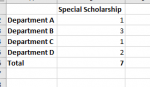
This formula is then repeated for each department (see image).

What do I need to add so that I only count the first seven occurences of 'Schol List'!$F$28:$F$61,"*YES*" regardless of department?
 

Attachments

  • Capture.PNG
    Capture.PNG
    3.7 KB · Views: 11

Excel Facts

How to find 2nd largest value in a column?
MAX finds the largest value. =LARGE(A:A,2) will find the second largest. =SMALL(A:A,3) will find the third smallest
Welcome to the forum!

How about:

Book1.xlsx
ABCDEF
1Special Scholarship
2Department A1
3Department B3
4Department C1
5Department D2
6Total7
7
27
28Department AYes
29Department BYes
30Department BYes
31xxYes
32Department CYes
33Department DYes
34Department BYes
35Department DYes
36Department DYes
37Department DYes
Schol List
Cell Formulas
RangeFormula
B2:B5B2=MIN(COUNTIFS('Schol List'!$F$28:$F$61,"*YES*",'Schol List'!$C$28:$C$61,A2),7-SUM(B$1:B1))
B6B6=SUM(B2:B5)
 
Last edited:
Upvote 0
Welcome to the forum!

How about:

Book1.xlsx
ABCDEF
1Special Scholarship
2Department A1
3Department B3
4Department C1
5Department D2
6Total7
7
27
28Department AYes
29Department BYes
30Department BYes
31xxYes
32Department CYes
33Department DYes
34Department BYes
35Department DYes
36Department DYes
37Department DYes
Schol List
Cell Formulas
RangeFormula
B2:B5B2=MIN(COUNTIFS('Schol List'!$F$28:$F$61,"*YES*",'Schol List'!$C$28:$C$61,A2),7-SUM(B$1:B1))
B6B6=SUM(B2:B5)

Hi Eric,

Thanks. I can't seem to get this to work for me.

Maybe if I share a something more similar to what I am actually working on:

RankDepartment AApplicant SummarySpecial Scholarship
1​
Department AXXXYes
2​
Department BXXX
3​
Department AXXXYes
4​
Department CXXX
5​
Department AXXXYes
6​
Department DXXX
7​
Department CXXX
8​
Department CXXXYes
9​
Department AXXX
10​
Department BXXX
11​
Department DXXXYes
12​
Department AXXXYes
13​
Department CXXXYesDepartment Special Scholarship
14​
Department AXXXDepartment A
15​
Department AXXXYesDepartment B
16​
Department BXXXDepartment C
17​
Department BXXXDepartment D
18​
Department AXXX
19​
Department DXXXYes
20​
Department DXXXYes
21​
Department CXXX
22​
Department AXXXYes
23​
Department BXXXYes

I want the Table on the right to count the those eligible for the special scholarship up to seven. Does this make sense?
 
Upvote 0
Book1.xlsx
ABCDEFG
1RankDepartment AApplicant SummarySpecial ScholarshipDepartmentSpecial Scholarship
21Department AXXXYesDepartment A4
32Department BXXXDepartment B0
43Department AXXXYesDepartment C2
54Department CXXXDepartment D1
65Department AXXXYes7
76Department DXXX
87Department CXXX
98Department CXXXYes
109Department AXXX
1110Department BXXX
1211Department DXXXYes
1312Department AXXXYes
1413Department CXXXYes
1514Department AXXX
1615Department AXXXYes
1716Department BXXX
1817Department BXXX
1918Department AXXX
2019Department DXXXYes
2120Department DXXXYes
2221Department CXXX
2322Department AXXXYes
2423Department BXXXYes
Sheet9
Cell Formulas
RangeFormula
G2:G5G2=COUNTIFS(B$2:INDEX(B:B,SMALL(IF(D:D="Yes",ROW(D:D)),7)),F2,D$2:INDEX(D:D,SMALL(IF(D:D="Yes",ROW(D:D)),7)),"Yes")
G6G6=SUM(G2:G5)
Press CTRL+SHIFT+ENTER to enter array formulas.
 
Upvote 0
I understand what you want is:
counting from D2 untile the seventh Yes appears, for example, D2:D14 contains 7 Yes, then count the number of each department which meet two criterias: B:B=department name and D2:D14=Yes. if my understanding is right, my post #4 is one of the solutions.
 
Upvote 0
Book1.xlsx
ABCDEFG
1RankDepartment AApplicant SummarySpecial ScholarshipDepartmentSpecial Scholarship
21Department AXXXYesDepartment A4
32Department BXXXDepartment B0
43Department AXXXYesDepartment C2
54Department CXXXDepartment D1
65Department AXXXYes7
76Department DXXX
87Department CXXX
98Department CXXXYes
109Department AXXX
1110Department BXXX
1211Department DXXXYes
1312Department AXXXYes
1413Department CXXXYes
1514Department AXXX
1615Department AXXXYes
1716Department BXXX
1817Department BXXX
1918Department AXXX
2019Department DXXXYes
2120Department DXXXYes
2221Department CXXX
2322Department AXXXYes
2423Department BXXXYes
Sheet9
Cell Formulas
RangeFormula
G2:G5G2=COUNTIFS(B$2:INDEX(B:B,SMALL(IF(D:D="Yes",ROW(D:D)),7)),F2,D$2:INDEX(D:D,SMALL(IF(D:D="Yes",ROW(D:D)),7)),"Yes")
G6G6=SUM(G2:G5)
Press CTRL+SHIFT+ENTER to enter array formulas.

This looks like it is doing exactly what I want but I'm getting a #NUM! error. Even when I am copying your entire spreadsheet.

Apologies if this is a bit of a basic question.
 
Upvote 0
I think after looking at your latest example, and shaowu459's formula, I think he has the right idea. Here's another formula which does the same thing but doesn't require array entry:

G2:G5: =SUMPRODUCT(--(B$2:B$24=F2),--(D$2:D$24="yes"),--(ROW(B$2:B$24)<=AGGREGATE(15,6,ROW(D$2:D$24)/(D$2:D$24="yes"),7)))
 
Upvote 0
This looks like it is doing exactly what I want but I'm getting a #NUM! error. Even when I am copying your entire spreadsheet.

Apologies if this is a bit of a basic question.
will you please upload a screenshot to show the error? make the editing bar visible so I can see the formula.
 
Upvote 0
I think after looking at your latest example, and shaowu459's formula, I think he has the right idea. Here's another formula which does the same thing but doesn't require array entry:

G2:G5: =SUMPRODUCT(--(B$2:B$24=F2),--(D$2:D$24="yes"),--(ROW(B$2:B$24)<=AGGREGATE(15,6,ROW(D$2:D$24)/(D$2:D$24="yes"),7)))

Thanks this works perfectly.

Only trouble is I am actually working on a sheet that doesn't have 'Department A' listed against each Row. Instead I have a complicatd index which is "Department_ID Number" eg Department A would be "DA_12345678" and I can't seem to work out how to do the partial string search that I had been using - eg "*DA*" in previous forumlas. Wish I could share my sheet but too much sensitive data.

I was also hoping to simply put this into Google Sheets but of course it doesnt have the Aggregate formula in Sheets - one of the many issues with organisations encouraging staff to use Google Programs.
 
Upvote 0
1590464393166.png

Book1.xlsx
ABCDEFG
1RankDepartment AApplicant SummarySpecial ScholarshipDepartmentSpecial Scholarship
21Department AXXXYesDepartment A4
32Department BXXXDepartment B0
43Department AXXXYesDepartment C2
54Department CXXXDepartment D1
65Department AXXXYes7
76Department DXXX
87Department CXXX
98Department CXXXYes
109Department AXXX
1110Department BXXX
1211Department DXXXYes
1312Department AXXXYes
1413Department CXXXYes
1514Department AXXX
1615Department AXXXYes
1716Department BXXX
1817Department BXXX
1918Department AXXX
2019Department DXXXYes
2120Department DXXXYes
2221Department CXXX
2322Department AXXXYes
2423Department BXXXYes
Sheet9
Cell Formulas
RangeFormula
G2:G5G2=COUNTIFS(B$2:INDEX(B:B,SMALL(IF(D:D="Yes",ROW(D:D)),7)),F2,D$2:INDEX(D:D,SMALL(IF(D:D="Yes",ROW(D:D)),7)),"Yes")
G6G6=SUM(G2:G5)
Press CTRL+SHIFT+ENTER to enter array formulas.
 
Upvote 0

Forum statistics

Threads
1,215,507
Messages
6,125,207
Members
449,214
Latest member
mr_ordinaryboy

We've detected that you are using an adblocker.

We have a great community of people providing Excel help here, but the hosting costs are enormous. You can help keep this site running by allowing ads on MrExcel.com.
Allow Ads at MrExcel

Which adblocker are you using?

Disable AdBlock

Follow these easy steps to disable AdBlock

1)Click on the icon in the browser’s toolbar.
2)Click on the icon in the browser’s toolbar.
2)Click on the "Pause on this site" option.
Go back

Disable AdBlock Plus

Follow these easy steps to disable AdBlock Plus

1)Click on the icon in the browser’s toolbar.
2)Click on the toggle to disable it for "mrexcel.com".
Go back

Disable uBlock Origin

Follow these easy steps to disable uBlock Origin

1)Click on the icon in the browser’s toolbar.
2)Click on the "Power" button.
3)Click on the "Refresh" button.
Go back

Disable uBlock

Follow these easy steps to disable uBlock

1)Click on the icon in the browser’s toolbar.
2)Click on the "Power" button.
3)Click on the "Refresh" button.
Go back
Back
Top