Create a validation alert within a cell based on two conditions being true

[Silver870]

First, thanks for reading my post!

So here goes, I'm trying to setup either a formula or macro, whichever would work best, in which if two conditions hold true, both based off a partial text search function, a validation alert comes up for that cell. The conditions vary. So as an example:

if cell A2 contains "Meeting"
and cell C2 contains "Foyer"
Change cell C2's color to pink and add a validation alert to cell C2 saying "Change to "Meeting"

Or

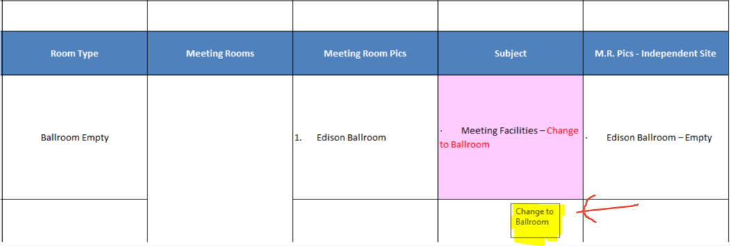
if cell A3 contains "Ballroom"
and cell C3 contains "Meeting"
Change cell C3's color to pink and add a validation alert to cell C3 saying "Change to "Ballroom".

I've gotten the color to change using conditional formatting with an "And" function combined with a "Search" function, but I don't know how to get the validation alert added to the cell. I was thinking maybe I could run a validation rule based off any cells that are the specific color that they would change to, but that doesn't appear to be a validation option. Also, the validation text alert would vary depending on the circumstance as illustrated in my example above, where in the first case, the alert says to change it to "Meeting" and in the second case, it says to switch it to "Ballroom". This is typically dependent on whatever is found in column A, so perhaps another if statement could be setup whereby:
if a cell in column c is pink, the alert would state "Change to Meeting", but only if the word "Meeting" is what is found through a partial text search in column A. And if "Ballroom" was found in column A, it would state "Change to Ballroom".

Once this is built out, I then want to report on how many times I've provided the validation alert across a specific range. I'm thinking I can use a CountIf formula or something similar to do that, but let me know if you agree.

Thanks so much for your help!

 

[oldbrewer]

please define what you mean by validation alert...do you mean a note....

 

[Silver870]

please define what you mean by validation alert...do you mean a note....

Hi @oldbrewer,
Thanks for the quick response! So I'm trying to create a validation input message, that appears when you click on the cell if both conditions are true. In addition, I want the cell to turn pink, again if both conditions are true, so the person I'm sending edits to quickly and easily knows which cells to update. I've been able to accomplish this on one cell, using a combination of conditional formatting and the validation tool. I've used the formula:
=AND(SEARCH("*Meeting*",F8),SEARCH("*Ballroom*",C8))

And I can get the conditional formatting to work across a range of cells, except in a case where two cells are merged. I'd like to figure out how to fix this as well. But when I try to include a range in the formula for the validation input message, shown below, I get an error and the formula doesn't work:
=AND(SEARCH("*Meeting*",F8:F20),SEARCH("*Ballroom*",G8:G20))

Below is a screenshot of what I'm trying to accomplish. Sorry it's so big. For whatever reason I can't seem to resize it.

And here is a sample spreadsheet which shows what I've included in my screen shot.

https://drive.google.com/open?id=0Bx_7oQCiOLjSWmVfX0N2Sm8yLWM

Thanks for your help!

 

[oldbrewer]

what is a validation alert

a cell contains say "ballroom" and a note can be added - visible only when you hover over the cell - or an adjacent cell normally blank can display a message - still not sure what you want...

 

[Silver870]

Hi @OldBrewer:

Sorry for any confusion. The note you receive when you hover over the cell is what I'm referring to. If you go to the spreadsheet I sent, you'll see I've set this up already in row 8.

Excel seems to refer to this note as "Input Message". You'll locate it when you click on the Data tab and then click on Data Validation. It's the second tab within the Data Validation window.

Let me know if you have any additional questions.

Thanks!

Dan

 

[oldbrewer]

AH !!! you can have a note that appears when you hover over a cell and an input message when you select the cell....

so are you wanting, when certain defined cell values occur to color a cell to draw attention to it, so that you know to click it to read the validation message ?

 

[Silver870]

AH !!! you can have a note that appears when you hover over a cell and an input message when you select the cell....

so are you wanting, when certain defined cell values occur to color a cell to draw attention to it, so that you know to click it to read the validation message ?

Exactly!

That's why the same formula can be used for both. I just need to extend the range, and account for the different scenarios, which I think I can do using an "OR" function, verses having multiple "AND" functions. Where I'm stuck is trying to extend the range so it comes 2500 rows.

 

[oldbrewer]

let us say you want cells in column A to colour if either cell D or cell E is zero

	foyer		5	0
					this conditional format turns A1 red if either d1 or E1 = 0
					=OR(D1=0,E1=0)
					when you click on cell A1 which is now red
					you get the message
					please change cell B1 to ballroom

<colgroup><col span="12"></colgroup><tbody>
</tbody>

 

[Silver870]

Morning,

Looks like you had a late night!

Thanks for the thoughtful responses!!!

I totally understand what you're saying. My challenge is that the conditional value is based off of a partial text statement, not a number, and as a partial text statement, I've setup the formula so it's only searching for some of the text within a given cell, not all the text, which is why I used the search function.

I believe an alternative function to make this work would be "Match", which I was playing with last night.

So back to what I was saying, if cell A states "Meeting Room" and cell B states "Ballroom empty", the formula would only search for "Meeting" in cell A and "Ballroom" in cell B. My thought is to then apply an Or function to the formula for additional conditions I'd want the formula to search for and identify, turning the cell pink and adding a note, if the condition was found. So alternative conditions might be:
- cell A contains "Ballroom" and cell B contains "Meeting"
- cell A contains "Ballroom" and cell B contains "Foyer"

So on and so forth.

So all that being said, I'm running into an issue applying the condition to a given cell if the cell is referencing a merged cell. So to give further clarity on the merged cell issue, if you go back to the spreadsheet example I sent, you'll see that there are instances where multiple rows are merged. If a cell is merged across two rows, so let's say I've merged cells A3:A4, the conditional formula will apply to cell B3, but not B4. I need it to apply to both. And then I also need the formula to apply to a large range of rows and worked with a merged row and a non-merged row. So as an example of the total range, it could be from A8:A:2500 and B8:B2500. For whatever reason, whenever I try and apply a range to the formula,the formula stops working. Any idea on how to fix these concerns?

Thanks so much for all your time and consideration!

Dan

 

[oldbrewer]

4	7
	8
	9
5	10
	11
	12
				A1 A2 A3 are merged
				A4,A5,A6 are merged
				I applied conditional formatting to B1
				and used format painter to apply it to B2:B6 and the 2 merged cells in col A
				are you trying to do something else ?

<colgroup><col span="13"></colgroup><tbody>
</tbody>