Determining amounts when a cell may represent more than one item

[IamBatman]

I'm not quite sure how to explain this properly (and the title is probably rubbish), so please also look at the picture.

I have a list of dimensions from projects that I've combined into one spreadsheet. I need to be able to see what size pieces we end up with the most, but some of the lines represent more than one piece.

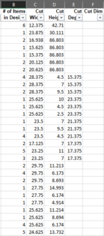
For example. If I want to determine how many items have 7 as one of their dimensions, I can use countif(C:E,"7") (except I usually use a cell reference instead of the actual dimension). From the set shown, I'll get back 4, but there are really 8 pieces (quantities of 2, 1, 2, and 3). How do I account for the item numbers in column B?

I thought briefly about manually correcting this (insert line(s), copy the dimensions, and change # of items to one), but 536 of 930 lines have more than 1 item in the design, and 22 have 10 or more items in the design. I wouldn't mind them showing like that (quantity of 1), but I'm not taking that much time. I'm also fine with using something besides countif. I'm really just looking for something simple (I can set it up once and keep adding data) and as automated as possible.

Does anyone have any suggestions?
Thanks

 

[jtakw]

Hi,

May be this might do what you want:

Book3.xlsx
	A	B	C	D	E	F	G
1						Look for	Total Count
2	2	11	7	101		7	8
3	2	12	5	102
4	1	13	7	103
5	1	14	4	104
6	1	15	3	105
7	1	16	2	106
8	1	17	1	107
9	2	18	7	108
10	2	19	8	109
11	2	20	9	110
12	2	21	10	111
13	2	22	11	112
14	3	23	7	113
15	3	24	2	114
Sheet1027

Cell Formulas
Range	Formula
G2	G2	=SUMPRODUCT((B2:E100=F2)*A2:A100)

 

[BSALV]

if it was arranged in a table (here tabel1)

Map1
	B	C	D	E	F	G
1	B	C	D	E
2	1	7				5
3	1		7
4	1			7
5	1		5
6	2	7	7	7
7
8
9
10
Blad1

Cell Formulas
Range	Formula
G2	G2	=SUM((COUNTIF(OFFSET(Tabel1[[#Headers],[C]:[E]],SEQUENCE(ROWS(Tabel1[B])),,,),7)>0)*Tabel1[B])

 

[Eric W]

How about:

Book1
	A	B	C	D	E	F	G	H	I	J	K
1	# of items	Width	Height	Depth	Dim
2	6	9	10	11
3	1	9	10	11			Dimension	Column	Count		All columns
4	2	9	10	7			7	Height	8		11
5	1	7	10	11
6	1	9	10	11
7	2	9	10	11
8	2	9	10	11
9	4	9	10	11
10	2	9	7	11
11	2	9	10	11
12	1	9	10	11
13	1	9	10	11
14	1	9	10	11
15	1	9	7	11
16	1	9	10	11
17	4	9	10	11
18	2	9	7	11
19	5	9	10	11
20	3	9	7	11
21	2	9	10	11
22	4	9	10	11
23	2	9	10	11
24	1	9	10	11
25	1	9	10	11
26	1	9	10	11
27	1	9	10	11
28	1	9	10	11
29	1	9	10	11
30	4	9	10	11
31	5	9	10	11
Sheet2

Cell Formulas
Range	Formula
I4	I4	=SUMPRODUCT(A2:A31*(INDEX(B2:D31,0,MATCH(H4,B1:D1,0))=G4))
K4	K4	=SUMPRODUCT(A2:A31*SIGN(MMULT(--(B2:D31=G4),{1;1;1})))

 

[BSALV]

#2 vs #3 : if you have in the same row 2 or 3 7's, do you have to calculate that as 1 or as 2 or 3 ?

 

[IamBatman]

Hi,

May be this might do what you want:

Book3.xlsx
	A	B	C	D	E	F	G
1						Look for	Total Count
2	2	11	7	101		7	8
3	2	12	5	102
4	1	13	7	103
5	1	14	4	104
6	1	15	3	105
7	1	16	2	106
8	1	17	1	107
9	2	18	7	108
10	2	19	8	109
11	2	20	9	110
12	2	21	10	111
13	2	22	11	112
14	3	23	7	113
15	3	24	2	114
Sheet1027

Cell Formulas
Range	Formula
G2	G2	=SUMPRODUCT((B2:E100=F2)*A2:A100)

I altered it slightly (added $ to the ranges, and went through 10000 instead of 100).

Works beautifully and simply. Thank you!

And thank you all for all the options.

 

[BSALV]

i preferred #4 as solution, simple !
What happens if there are multiple 7's in those 3 cells, is the result still okay ?

 

[IamBatman]

i preferred #4 as solution, simple !
What happens if there are multiple 7's in those 3 cells, is the result still okay ?

You mean like 77? Or something else?


I've had issues with index and match sometimes, so I tend to avoid it.

This sheet won't be used tons. It was used to attempt to prove a point by showing what the data is, and may be used thusly again, but it's definitely not in daily use.

 

[BSALV]

column E = manual calculation and sum in J4
H4 = Erik W
I4 = Jtakw
the problem is row 4, multiple 7's in the same row !
For Erik W those 3 7's count as 1, for Jtakw as 3, multiplied by 2 (cell A4) is that 2 or 6 ???
Is it possible to have multiple 7's in a row ?

Batch_Example.xlsx
	A	B	C	D	E	F	G	H	I	J
1	# of items	Width	Height	Depth	formula
2	6	9	10	11	0
3	1	9	10	11	0		Dimension	ErikW	Jtakw	check
4	2	7	7	7	2		7	12	16	12
5	1	7	10	11	1
6	1	9	7	11	1
7	2	9	10	11	0
8	2	9	10	11	0
9	4	9	10	11	0
10	2	9	7	11	2
11	2	9	10	11	0
12	1	9	10	11	0
13	1	9	10	11	0
14	1	9	10	11	0
15	1	9	7	11	1
16	1	9	10	11	0
17	4	9	10	11	0
18	2	9	7	11	2
19	5	9	10	11	0
20	3	9	7	11	3
21	2	9	10	11	0
22	4	9	10	11	0
23	2	9	10	11	0
24	1	9	10	11	0
25	1	9	10	11	0
26	1	9	10	11	0
27	1	9	10	11	0
28	1	9	10	11	0
29	1	9	10	11	0
30	4	9	10	11	0
31	5	9	10	11	0
32
Blad2

Cell Formulas
Range	Formula
H4	H4	=SUMPRODUCT(My_Items*SIGN(MMULT(--(My_Sizes=G4),{1;1;1})))
I4	I4	=SUMPRODUCT((My_Sizes=G4)*My_Items)
J4	J4	=SUM(E2:E31)
E2:E31	E2	=A2*(COUNTIF(A2:D2,$G$4)<>0)

Named Ranges
Name	Refers To	Cells
My_Items	=Blad2!$A$2:$A$31	H4:I4, E2
My_Sizes	=Blad2!$B$2:$D$31	E2, H4:I4

Cells with Conditional Formatting
Cell	Condition		Cell Format	Stop If True
B2:F31	Expression	=$G$4=B2	text	NO

 

[Peter_SSs]

I was also wondering about the same dimension occurring in multiple columns on the same row.

22 03 02.xlsm
	A	B	C	D	E	F	G	H
1	# of items	Width	Height	Depth
2	6	9	11	11
3	1	11	10	11			Dimension	Items
4	2	7	7	7			7	6
5	1	7	10	8			11	9
6	1	9	7	8
7	2	9	10	7
8	2	9	10	11
9
Count Items

Cell Formulas
Range	Formula
H4:H5	H4	=SUM(FILTER(A$2:A$10000,(B$2:B$10000=G4)+(C$2:C$10000=G4)+(D$2:D$10000=G4),0))