Display and count unique values in date range

[alfik1]

Hi all,

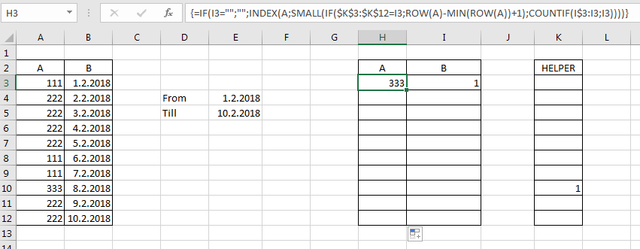
Im standing in front of the task (see picture attached) and I cannot to figure it out . Does anybody has idea how to achieve desired result based on the criterias defined?
The result should be done by fromula, not by pivot or vba. If possible, do not use any formula in data table...
Im using excel 2016
Many thanx for any idea

 

[alfik1]

If its easier to get result with text in A column, no problem, it can be text there...

 

[Marcelo Branco]

I'm trying to create a not very complicated formula. Thinking about.

M.

 

[alfik1]

I'm trying to create a not very complicated formula. Thinking about.

M.

And is possible that helper column will be a part of result table and not data table?

 

[Marcelo Branco]

Maybe something like this

A​

B​

C​

D​

E​

F​

G​

H​

I​

J​

K​

L​

1​

Data​

Results​

2​

A​

B​

From​

01/02/2018​

Code​

Top 10​

Helper​

3​

111​

01/02/2018​

Till​

10/02/2018​

222​

6​

3​

4​

222​

02/02/2018​

111​

3​

6​

5​

222​

03/02/2018​

333​

1​

6​

222​

04/02/2018​

7​

222​

05/02/2018​

8​

111​

06/02/2018​

9​

111​

07/02/2018​

10​

333​

08/02/2018​

1​

11​

222​

09/02/2018​

12​

222​

10/02/2018​

13​

14​

15​

16​

17​

18​

19​

20​

21​

22​

23​

<tbody>
</tbody>

Helper column
Formula in K3 copied down for some rows (say until row 22 --->gray area)
=IFERROR(IF(COUNTIF(INDEX(Data[A],1):Data[@A],Data[@A])=1,COUNTIFS(Data[A],Data[A],Data,">="&F$2,Data,"<="&F$3),""),"")

Formula in I3 copied down
=IF(COUNTIF(K$3:K$22,">="&LARGE(K$3:K$22,MIN(COUNT(K$3:K$22),10)))>=ROWS(I$3:I3),LARGE(K$3:K$22,ROWS(I$3:I3)),"")

Array formula in H3 copied down
=INDEX(Data[A],SMALL(IF(K$3:K$22=I3,ROW(Data[A])-MIN(ROW(Data[A]))+1),COUNTIF(I$3:I3,I3)))
Ctrl+Shift+Enter, not just Enter

M.

 

[Marcelo Branco]

oops...

Adjustments
Array formula in I3 copied down
=IFERROR(IF(COUNTIF(K$3:K$22,">="&LARGE(K$3:K$22,MIN(COUNT(K$3:K$22),10)))>=ROWS(I$3:I3),LARGE(IF(ISNUMBER(K$3:K$22),IF(K$3:K$22>0,K$3:K$22)),ROWS(I$3:I3)),""),"")
Ctrl+Shift+Enter, not just Enter

Array formula in H3 copied down
=IF(I3="","",INDEX(Data[A],SMALL(IF(K$3:K$22=I3,ROW(Data[A])-MIN(ROW(Data[A]))+1),COUNTIF(I$3:I3,I3))))
Ctrl+Shift+Enter, not just Enter

M.

 

[alfik1]

Hi Marcelo, Im sending you result. I probably messed up something



Formulas used:

H3 (with Ctrl+Shift+Enter):

=IF(I3="";"";INDEX(A;SMALL(IF($K$3:$K$12=I3;ROW(A)-MIN(ROW(A))+1);COUNTIF(I$3:I3;I3))))

I3 (with Ctrl+Shift+Enter):

=IFERROR(IF(COUNTIF(K$3:K$12;">="&LARGE(K$3:K$12;MIN(COUNT(K$3:K$12);10)))>=ROWS(I$3:I3);LARGE(IF(ISNUMBER(K$3:K$12);IF(K$3:K$12>0;K$3:K$12));ROWS(I$3:I3));"");"")

K3:

=IFERROR(IF(COUNTIF(INDEX(A;1):A;A)=1;COUNTIFS(A;A;B;">="&E$4;B;"<="&E$5);"");"")

 

[Marcelo Branco]

Try (new version)

	A​	B​	C​	D​	E​	F​	G​	H​	I​	J​	K​
1​
2​	A​	B​						A​	B​		Helper​
3​	111​	01/02/2018​						222​	6​		3​
4​	222​	02/02/2018​		From​	01/02/2018​			111​	3​		6​
5​	222​	03/02/2018​		To​	10/02/2018​			333​	1​
6​	222​	04/02/2018​
7​	222​	05/02/2018​
8​	111​	06/02/2018​
9​	111​	07/02/2018​
10​	333​	08/02/2018​									1​
11​	222​	09/02/2018​
12​	222​	10/02/2018​
13​

<tbody>
</tbody>

Helper
Formula in K3 copied down until, say, K100
=IF(A3="","",IF(COUNTIF(A$3:A3,A3)=1,COUNTIFS(A$3:A$100,A3,B$3:B$100,">="&E$4,B$3:B$100,"<="&E$5),""))

Formula in I3 copied down until you get a blank
=IF(COUNTIF(K$3:K$100,">0")>=ROWS(I$3:I3),LARGE(K$3:K$100,ROWS(I$3:I3)),"")

Array formula in H3 copied down
=IF(I3="","",INDEX(A$3:A$100,SMALL(IF(K$3:K$100=I3,ROW(K$3:K$100)-ROW(K$3)+1),COUNTIF(I$3:I3,I3))))
Ctrl+Shift+Enter

M.

 

[alfik1]

The columns I and K seems working, but H shows this:

 

[Marcelo Branco]

Select H3:H100
Delete
Select just H3 and re-enter formula in H3
copy down

M.

 

[alfik1]

Select H3:H100
Delete
Select just H3 and re-enter formula in H3
copy down

M.

heh, it works. Thank you.
And how the formula should looks like when the date E4 and E5 is in other sheet? I tried just point with mouse to other sheet, but it is not working...