Display unique values from Column based on Criteria of Another Column

[gldurand]

Hi There,

I am using Excel 2016

I have a huge dataset 30 col/1000 rows but 2 specific ones that i need to use for this task i think.

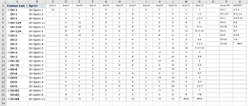
This is the PIVOT showing the data, but there are a number of duplicates in SPRINT

I want to be able to put into the cells for each issue key the unique Sprints associated to them

1) I want to remove the prefix and only put the numerical value)
2) The source data changes daily
3) I would prefer a formula (Even if i need to use helper columns) but VBA is Fine

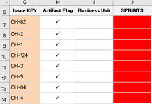
Here is my staging area where i want my result J7.. J8 etc....

Any help would certainly save me a huge amount of manual work.

THanks alot

 

[fjns]

Hi, see the linked file (with 12 auxiliary columns) for a possible solution...

The formulas used in the table:
C2: =MAX(I:I)
D2: =RIGHT(B2,LEN(B2)-10)
E2: =VALUE(D2)
F2: =COUNTIF(A:A,A2)
G2: =IF(COUNTIF(A$2:A2,A2)=F2,F2,0)
H2: =IF(COUNTIF(A$2:A2,A2)=1,1,0)
I2: =IF(COUNTIF(A$2:A2,A2)=1,SUM(H$2:H2)+1,0)
J2: =COUNTIFS(A:A,A2,E:E,"<"&E2)
K2: =IF(COUNTIF(A$2:A2,A2)=1,SUM(G$2:G2)+2,0)
L2: =MAX(K$2:K2)+J2
M2: =INDEX(D:D,MATCH(ROW(),L:L,0))
N2: =IF(H2=1,M2,N1&"-"&M2)
P2: =IF(ROW()>C$2,"",INDEX(A:A,MATCH(ROW(),I:I,0)))
Q2: =IF(ROW()>C$2,"",INDEX(N:N,MATCH(ROW(),I:I,0)+INDEX(F:F,MATCH(ROW(),I:I,0))-1))

SPRINTS.xlsx

 

[gldurand]

Hi FJNS

Wow, lots of steps and work... thanks so much. I have moved your AUX columns to my spreadhsheet and made the necessary conversions, seems to be working when i have values in ALL but the only issue is that I could have blanks in both these columns.

 

[gldurand]

And i showed you the Source data that was sorted, but its not always the case,

Want to identify all the OH Keys in Feature link and extract all the Sprints that are part of it

Example

Here is a more realistic view of the data

 

[gldurand]

FJNS

Ignore 2 previous posts

I have simplified the source to use a PIVOT Table to eliminate blanks. But the last record reference OH-84 has only 1 Sprint and its giving me an #N/A

Any ideas

 

[fjns]

Sorry, my formula for K2 is wrong.

This is the correct formula for K2:
=IF(COUNTIF(A$2:A2,A2)=1,SUM(G$2:G2)+MIN(2,F2),0)

SPRINTS2.xlsx

 

[gldurand]

ROCK STAR!!!! Thanks so much for this solution...

 

[gldurand]

FJNS

I have figured out most of the formulas, but wanting to learn, if its not too much work, can you explain your mindset and how you are using the ones missing. GREAT WORK and NO RUSH

C2: =MAX(I:I) - Maximum number of FEATURE LINKS to be used in P2 & Q2
D2: =RIGHT(B2,LEN(B2)-10) - Strip off Sprint prefix
E2: =VALUE(D2) - Convert to Number from Text
F2: =COUNTIF(A:A,A2) - Count number of FEATURE LINK Records
G2: =IF(COUNTIF(A$2:A2,A2)=F2,F2,0) - Identify Last FEATURE LINK in range to be used in K2
H2: =IF(COUNTIF(A$2:A2,A2)=1,1,0) - Identify First FEATURE link in Range to be used in I2
I2: =IF(COUNTIF(A$2:A2,A2)=1,SUM(H$2:H2)+1,0)
J2: =COUNTIFS(A:A,A2,E:E,"<"&E2)
K2: =IF(COUNTIF(A$2:A2,A2)=1,SUM(G$2:G2)+2,0)
L2: =MAX(K$2:K2)+J2
M2: =INDEX(D:D,MATCH(ROW(),L:L,0))
N2: =IF(H2=1,M2,N1&"-"&M2) - Sequential account for Sprint occurences
P2: =IF(ROW()>C$2,"",INDEX(A:A,MATCH(ROW(),I:I,0))) - List unique FEATURE Link from PIVOT until the numbr of occurences is reached
Q2: =IF(ROW()>C$2,"",INDEX(N:N,MATCH(ROW(),I:I,0)+INDEX(F:F,MATCH(ROW(),I:I,0))-1)) - Display last occurrence of Sprint listing until the number of occurrences is reached

 

[fjns]

Hi, I created a new table for unsorted case and for blank cells.

The formulas used in the new table:
A2: =IF(OR(INDEX(work!A:A,ROW())="",INDEX(work!B:B,ROW())=""),"",INDEX(work!A:A,ROW()))
B2: =IF(OR(INDEX(work!A:A,ROW())="",INDEX(work!B:B,ROW())=""),"",INDEX(work!B:B,ROW()))
C2: =IF(A2="","",IF(COUNTIFS(A$2:A2,A2,B$2:B2,B2)=1,1,""))
D2: =SUM(C:C)+1
E2: =IF(A2="","",IF(C2=1,A2,""))
F2: =IF(A2="","",IF(C2=1,B2,""))
G2: =IF(A2="","",E2&"#"&F2)
H2: =IF(A2="","",D$2-COUNTIFS(G:G,">"&G2))
I2: =IF(ROW()>D$2,"",INDEX(E:E,MATCH(ROW(),H:H,0)))
J2: =IF(ROW()>D$2,"",INDEX(F:F,MATCH(ROW(),H:H,0)))
K2: =MAX(Q:Q)
L2: =IF(ROW()>D$2,"",RIGHT(J2,LEN(J2)-10))
M2: =IF(ROW()>D$2,"",VALUE(L2))
N2: =IF(ROW()>D$2,"",COUNTIF(I:I,I2))
O2: =IF(ROW()>D$2,"",IF(COUNTIF(I$2:I2,I2)=N2,N2,0))
P2: =IF(ROW()>D$2,"",IF(COUNTIF(I$2:I2,I2)=1,1,0))
Q2: =IF(ROW()>D$2,"",IF(COUNTIF(I$2:I2,I2)=1,SUM(P$2:P2)+1,0))
R2: =IF(ROW()>D$2,"",COUNTIFS(I:I,I2,M:M,"<"&M2))
S2: =IF(ROW()>D$2,"",IF(COUNTIF(I$2:I2,I2)=1,SUM(O$2:O2)+MIN(2,N2),0))
T2: =IF(ROW()>D$2,"",MAX(S$2:S2)+R2)
U2: =IF(ROW()>D$2,"",INDEX(L:L,MATCH(ROW(),T:T,0)))
V2: =IF(ROW()>D$2,"",IF(P2=1,U2,V1&"-"&U2))
X2: =IF(ROW()>K$2,"",INDEX(I:I,MATCH(ROW(),Q:Q,0)))
Y2: =IF(ROW()>K$2,"",INDEX(V:V,MATCH(ROW(),Q:Q,0)+INDEX(N:N,MATCH(ROW(),Q:Q,0))-1))

SPRINTSnew.xlsx
SPRINTSnew2.xlsx

 

[fjns]

FJNS

I have figured out most of the formulas, but wanting to learn, if its not too much work, can you explain your mindset and how you are using the ones missing. GREAT WORK and NO RUSH

C2: =MAX(I:I) - Maximum number of FEATURE LINKS to be used in P2 & Q2
D2: =RIGHT(B2,LEN(B2)-10) - Strip off Sprint prefix
E2: =VALUE(D2) - Convert to Number from Text
F2: =COUNTIF(A:A,A2) - Count number of FEATURE LINK Records
G2: =IF(COUNTIF(A$2:A2,A2)=F2,F2,0) - Identify Last FEATURE LINK in range to be used in K2
H2: =IF(COUNTIF(A$2:A2,A2)=1,1,0) - Identify First FEATURE link in Range to be used in I2
I2: =IF(COUNTIF(A$2:A2,A2)=1,SUM(H$2:H2)+1,0)
J2: =COUNTIFS(A:A,A2,E:E,"<"&E2)
K2: =IF(COUNTIF(A$2:A2,A2)=1,SUM(G$2:G2)+2,0)
L2: =MAX(K$2:K2)+J2
M2: =INDEX(D:D,MATCH(ROW(),L:L,0))
N2: =IF(H2=1,M2,N1&"-"&M2) - Sequential account for Sprint occurences
P2: =IF(ROW()>C$2,"",INDEX(A:A,MATCH(ROW(),I:I,0))) - List unique FEATURE Link from PIVOT until the numbr of occurences is reached
Q2: =IF(ROW()>C$2,"",INDEX(N:N,MATCH(ROW(),I:I,0)+INDEX(F:F,MATCH(ROW(),I:I,0))-1)) - Display last occurrence of Sprint listing until the number of occurrences is reached

I2: =IF(COUNTIF(A$2:A2,A2)=1,SUM(H$2:H2)+1,0) - cell of OH Key in column P
J2: =COUNTIFS(A:A,A2,E:E,"<"&E2) - index of Sprint per OH Key
K2: =IF(COUNTIF(A$2:A2,A2)=1,SUM(G$2:G2)+2,0) - first cell of OH Key in column A
L2: =MAX(K$2:K2)+J2 - cell of Sprint in column B
M2: =INDEX(D:D,MATCH(ROW(),L:L,0)) - Sprint occurences