DIV and VALUE error on IF ABS statement

[Helloitsme]

I'm having a couple issues with formulas which i'm not smart enough to solve, I hope someone will be able to help me, I've added the minisheet at the end of this wall of text

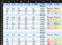
K to N is filled manually.

Error:
Q displays error "VALUE" if K or M is N/A, Q should remain blank in this case

Explanation
O is the average of K and M with round 0, formula =IF(COUNTA(K4;M4)=2;ROUND(AVERAGE(K4;M4);0);"")
Q is the difference between K and M with ABS, IF=0 leave blank, formula IF(ABS([K]-[M])=0;"";ABS([K]-[M]))

---------

Error:
P displays error DIV/0 if L and N is blank, P should remain blank in this case
R displays error VALUE if L or N is N/A, R should remain blank in this case

Explanation
P is the average of L and N with round 1 decimal, add /10 to the end, formula =ROUND(AVERAGE(L4;N4);1)&"/10"
R is the difference between L and N with ABS, IF=0 leave blank, formula IF(ABS([L]-[N])=0;"";ABS([L]-[N]))

Hope everyone has a great weekend!

Pricebook14JAN22.xlsx
	K	L	M	N	O	P	Q	R
1	CGR	CGT	CMCR	CMCT	AR	ATS	RD	TD
2						#DIV/0!
3	N/A	N/A	61	4.8	61	4,8/10	#VALUE!	#VALUE!
4	61	7	140	3.5	101	5,3/10	79	3.5
5	57	7	47	5.2	52	6,1/10	10	1.8
Listings

Cell Formulas
Range	Formula
O2:O5	O2	=IF(COUNTA(K2,M2)=2,ROUND(AVERAGE(K2,M2),0),"")
P2:P5	P2	=ROUND(AVERAGE(L2,N2),1)&"/10"
Q2:R5	Q2	=IF(ABS(K2-M2)=0,"",ABS(K2-M2))

Cells with Conditional Formatting
Cell	Condition		Cell Format	Stop If True
R1:R89	Cell Value	between 4,1 and 10	text	NO
R1:R89	Cell Value	between 2,1 and 4	text	NO
R1:R89	Cell Value	between 0 and 2	text	NO
Q1:Q89	Cell Value	between 51 and 500	text	NO
Q1:Q89	Cell Value	between 21 and 50	text	NO
Q1:Q89	Cell Value	between 0 and 20	text	NO

 

[Helloitsme]

I worked it out. DIV error could be fixed with IFERROR statement: =IFERROR(ROUND(AVERAGE(M2;O2);1)&"/10";"")
Value Error fixed with: =IF(OR(L3="";N3="");"";IFERROR(ABS(L3-N3);""))

 

[Peter_SSs]

.. or you could have continued with the 'COUNT' idea used in column O, but COUNT, not COUNTA. The advantage of this is that it would not hide other errors that you might actually want to know about.
Examples:

In P2: =IF(COUNT(L2;N2);ROUND(AVERAGE(L2;N2),1)&"/10";"")
In Q3: =IF(COUNT(K3;M3)=2;IF(ABS(K3-M3)=0;"";ABS(K3-M3));"")

 

[Helloitsme]

.. or you could have continued with the 'COUNT' idea used in column O, but COUNT, not COUNTA. The advantage of this is that it would not hide other errors that you might actually want to know about.
Examples:

In P2: =IF(COUNT(L2;N2);ROUND(AVERAGE(L2;N2),1)&"/10";"")
In Q3: =IF(COUNT(K3;M3)=2;IF(ABS(K3-M3)=0;"";ABS(K3-M3));"")

This was exactly the solutions I looked for, and no extra errors occoured after I implemented these two so I'm very content! Thank you Peter

 

[Peter_SSs]

You're welcome. Glad to help.