Dual Line Graph

[rcb007]

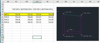
I am trying to figure out how to create a macro that can plot 4 points from 4 different cells, with a possible horizontal line connecting the points.

Example.
A1=100
A2=90
A3=103
A4=85

(A1)._______________.(A3)


(A2)._______________.(A4)


With that, I have several rows that have numbers like the above. How could I select a row and it plots the graph, if possible?

Thank you for any help!!

 

[sijpie]

Not clear on what you want to achieve.

I have several rows that have numbers like the above

do you mean several colums like the above (as A1:A4 is in one column)?


to get a graph like

you will need to split up each column in two columns

So that your
A1=100
A2=90
A3=103
A4=85

becomes
A1=100
A2=90
B1=103
B2=85

You could do that with a macro.

Does that help?

 

[rcb007]

I think you are definitely on the right track. I have attached a screen shot of (hopefully) a better diagram of showing what I would like to do wit the graph.

The Graph you showed above is exactly what I am wanting to do.

I would want to select (example pipe 1) the 4 cells (highlighted) and then be able to see the numbers in the graph form. If I select the pipe 3 line with the 4 cells, I would like to see those numbers on the graph.

I hope this makes it more clear.

 

[sijpie]

Here is what I have made

If the user selects a cell somewhere in the range of pipe coordinates, the graph will be modified for the row. So select AB22 and Pipe3 coordinates will be shown. Select AD20 and Pipe1 will be shown.

To make this work, you first need to create your graph. (Do this before you have copied the macros, else you will get endless error messages)
The easy way (showing incorrect lines, but that doesn't matter at this stage) is to select AC20:AD21. Then insert 2D line graph.

If you already have a graph, then ignore the above.

Note the name of your graph.

Paste the following code into a normal VBA module (press Alt-F8, then type in xx and Create... button. This will open the VBA editor. Delete the macro created, paste the below in instead)

Option Explicit

Sub ModifyGraphSource(wsWS As Worksheet, rR As Range)
' Adjust the series in a 2D line chart to the values
' given in the row provided by rR
' Also adjust the title of the graph

    Dim chChrt As ChartObject
    Dim rIn As Range, rStr1 As Range, rStr2 As Range
    
    If rR.Cells.Count > 1 Then Exit Sub 'Ignore if user selected several cells
    
    On Error GoTo NoChart
    Set chChrt = wsWS.ChartObjects("Chart 2") '<<<< Modify chartname as required
    On Error GoTo 0
    
    'from the selected cell, get the input row and the two ranges for the lines
    Set rIn = rR.CurrentRegion
    Set rIn = Range(Cells(rR.Row, rIn.Column), Cells(rR.Row, rIn.Column + rIn.Columns.Count - 1))
    Set rStr1 = rIn.Cells(1, 2).Resize(1, 2)
    Set rStr2 = rIn.Cells(1, 4).Resize(1, 2)

    'now update the chart
    With chChrt.Chart
        .SeriesCollection(1).Values = wsWS.Name & "!" & rStr1.Address
        .SeriesCollection(2).Values = wsWS.Name & "!" & rStr2.Address
        .ChartTitle.Caption = rIn.Cells(1, 1).Value
    End With
    Exit Sub
    
NoChart:
    MsgBox "The chart has not been found.", Buttons:=vbCritical + vbOKOnly
    On Error GoTo 0
End Sub

Notice in the comments (green) the comment starting with <<<<. Modify the chart name as to the one you have

Now go back to Excel and right click on the nametab of the sheet. Select view code...
This will open the code for this sheet. Insert the following code here:

Option Explicit

Private Sub Worksheet_SelectionChange(ByVal Target As Range)
    Const sAddress As String = "AB21"   '<<<< Left top corner of range with Pipe coordinates
    Dim rIn As Range
    
    'get the full range of all the piping coordinates
    Set rIn = Range(sAddress).CurrentRegion
    
    'check to see if the selected cell(s) is in this area
    If Not Intersect(Target, rIn) Is Nothing Then
        'selected cell is in piping coordinates area
        'so modify the graph
        ModifyGraphSource Me, Target
    End If
    
End Sub

That's it. Go back to Excel and select a cell in the range to see the graph being modified