Hi All,
Just joined the forum and the wealth of knowledge among the members, is extraordinary!
Which brings me onto a thread of my own to ask for some help:
I have been trying to apply for jobs in school as I worked in an Admin assistant and exams officer at a sixth form. However, the last 10 years I have been in retail management and now want to return back into the education sector. Anyway, over the lock down, I have applied for a number of roles and went as far as being shortlisted and progressed to interview. However, prior to the interview, the school sends out a few tasks to complete prior to interview and in almost all cases, there is an excel exercise. Recently, I did an exercise, but was so lost as to what functions to use, that I had to do the exercise manually and did not finish. After, I realised it was to do with vlookup and IF functions (or correct me if I'm wrong). Anyway, a few more applications that I had applied to, have got back to me yesterday and today for interview, and all 3 have said that there is an exercise, and I want to be ready if it is an excel exercise.
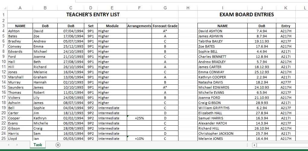
So in preparation, I was trying to do the excel task recently sent, it's a simple table with what the science department of a school entered for students and then another table beside, on the exam entries made to exam board. The exercise is:
On the excel spreadsheet there is an entry sheet received from the Science department asking you to confirm the pupils have been entered for the correct exam.
"As you will see, there are three possible tiers for this exam:
• Higher – Exam code – A217H.
• Intermediate – Exam code – A217I
• Foundation – Exam code – A217F
There is also a report printed from the Academy’s exam system confirming the actual entries sent to the exam board.
Please cross-check the two documents and identify whether pupils have been entered in accordance with the Science department’s wishes. Highlight in yellow any mistake or queries you might wish to discuss, and leave additional comments that explain what your queries are."
Here is a screenshot of the worksheet:
I attempted to do the exercise today. This is what I did:
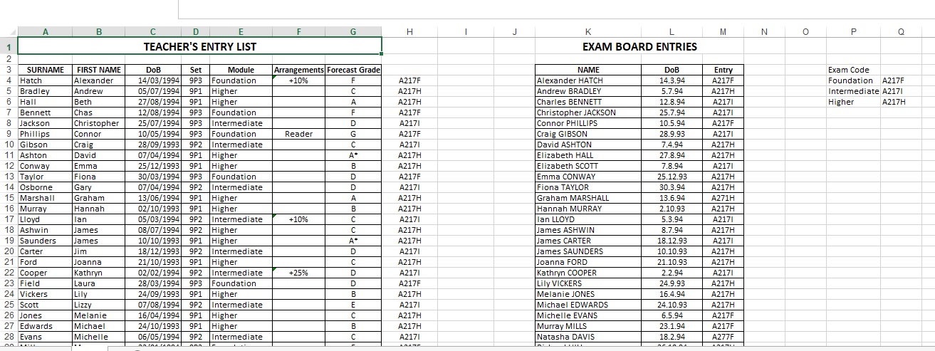
1. In Column H, entered the following formula: =VLOOKUP(E4, examcodes,2,FALSE), examcodes is the small table in columns Q and R. My thinking was that this will help check whether the students were entered for the correct module. See below:
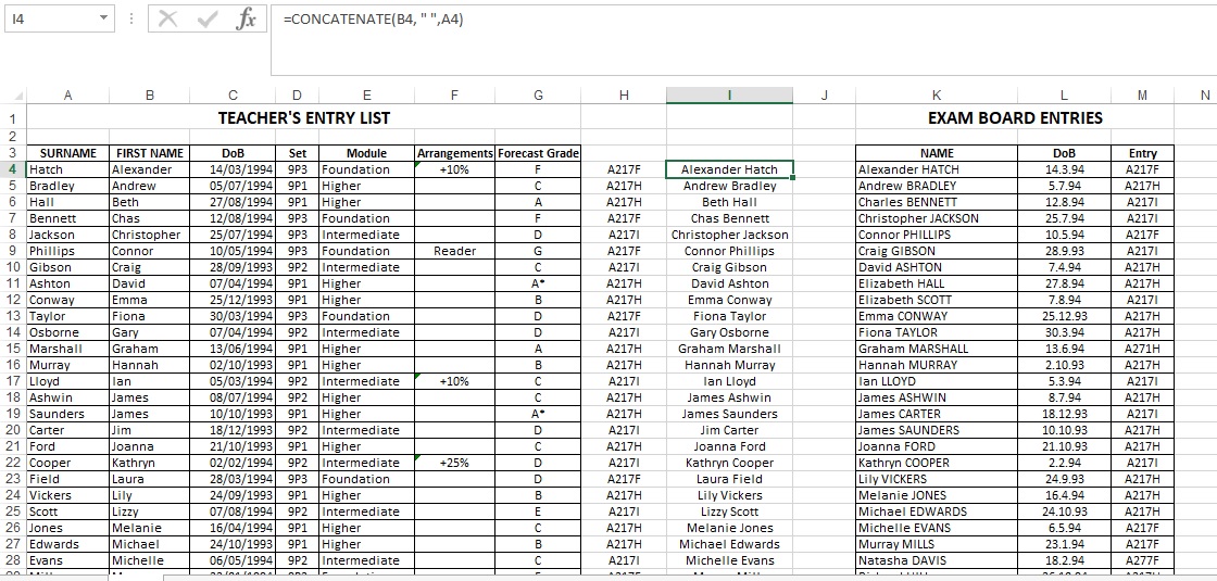
2. To check students name from Science dept list with exam board entries, I merged the first and last name to match the exam board entries name list, by using the following formula: =CONCATENATE(B4, " ",A4), in column I. See below:
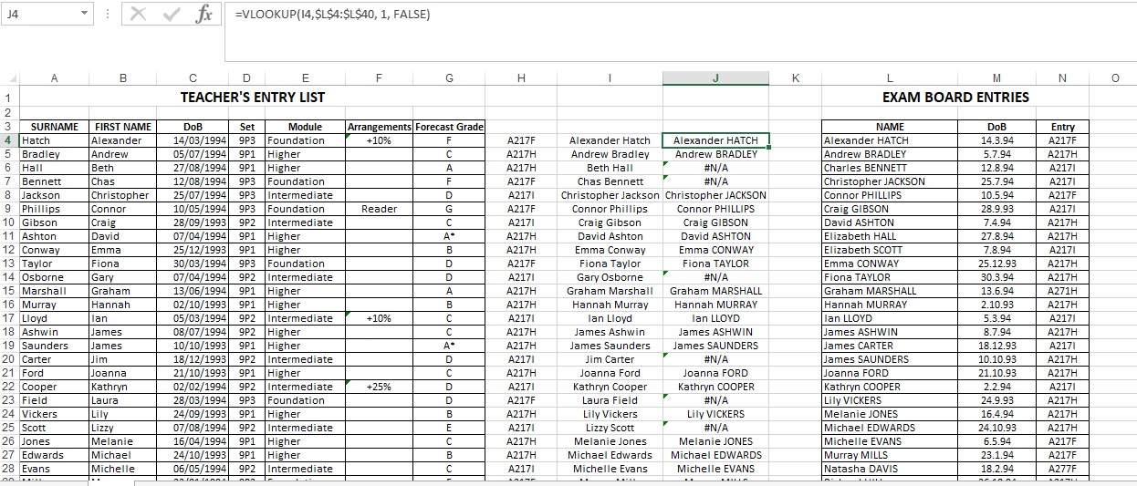
3. In column J, I then applied the formula: =VLOOKUP(I4,$L$4:$L$40, 1, FALSE), to cross-check the names from Science dept list against exam board entries. This produced NA for non-matching records. See below:
My questions are the following:
1. Is there a way of checking between the 2 tables in one go? And highlighting the records of name that do not appear in either table? For example, some records in exam entries table, use short hand names, like Jim instead of James, or Beth instead of Elizabeth.
2. How to check whether each student has been entered into the correct tier paper by name? I cannot figure this bit out and it is frustrating me, and feel like this is where the IF function comes into play.
3. Forgive me, but is there any better way to extract the data as required by the task?
I have not used excel in over 15 years and do not know where to start!
Thank you in advance ALL.
Jay
Just joined the forum and the wealth of knowledge among the members, is extraordinary!
Which brings me onto a thread of my own to ask for some help:
I have been trying to apply for jobs in school as I worked in an Admin assistant and exams officer at a sixth form. However, the last 10 years I have been in retail management and now want to return back into the education sector. Anyway, over the lock down, I have applied for a number of roles and went as far as being shortlisted and progressed to interview. However, prior to the interview, the school sends out a few tasks to complete prior to interview and in almost all cases, there is an excel exercise. Recently, I did an exercise, but was so lost as to what functions to use, that I had to do the exercise manually and did not finish. After, I realised it was to do with vlookup and IF functions (or correct me if I'm wrong). Anyway, a few more applications that I had applied to, have got back to me yesterday and today for interview, and all 3 have said that there is an exercise, and I want to be ready if it is an excel exercise.
So in preparation, I was trying to do the excel task recently sent, it's a simple table with what the science department of a school entered for students and then another table beside, on the exam entries made to exam board. The exercise is:
On the excel spreadsheet there is an entry sheet received from the Science department asking you to confirm the pupils have been entered for the correct exam.
"As you will see, there are three possible tiers for this exam:
• Higher – Exam code – A217H.
• Intermediate – Exam code – A217I
• Foundation – Exam code – A217F
There is also a report printed from the Academy’s exam system confirming the actual entries sent to the exam board.
Please cross-check the two documents and identify whether pupils have been entered in accordance with the Science department’s wishes. Highlight in yellow any mistake or queries you might wish to discuss, and leave additional comments that explain what your queries are."
Here is a screenshot of the worksheet:
I attempted to do the exercise today. This is what I did:
1. In Column H, entered the following formula: =VLOOKUP(E4, examcodes,2,FALSE), examcodes is the small table in columns Q and R. My thinking was that this will help check whether the students were entered for the correct module. See below:
2. To check students name from Science dept list with exam board entries, I merged the first and last name to match the exam board entries name list, by using the following formula: =CONCATENATE(B4, " ",A4), in column I. See below:
3. In column J, I then applied the formula: =VLOOKUP(I4,$L$4:$L$40, 1, FALSE), to cross-check the names from Science dept list against exam board entries. This produced NA for non-matching records. See below:
My questions are the following:
1. Is there a way of checking between the 2 tables in one go? And highlighting the records of name that do not appear in either table? For example, some records in exam entries table, use short hand names, like Jim instead of James, or Beth instead of Elizabeth.
2. How to check whether each student has been entered into the correct tier paper by name? I cannot figure this bit out and it is frustrating me, and feel like this is where the IF function comes into play.
3. Forgive me, but is there any better way to extract the data as required by the task?
I have not used excel in over 15 years and do not know where to start!
Thank you in advance ALL.
Jay


