Excel formatting everything lands in Column A

[nobailjustjail]

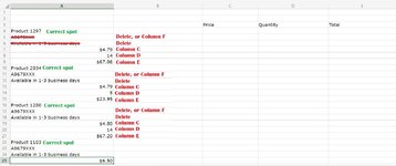
I am copy/pasting data from my suppliers website (from the checkout cart page).

When pasting into Excel it all goes into Column A (and some unnecessary info into Column B too but that is easily deleted).

I need a fast way to get the data into the correct columns as I am doing this on a very big scale.

I have tried using the ''Find All'' function as this would help me to remove the rows I want deleted. But it doesn't allow me to go ahead and highlight them all and deleted them all in one go after I have found them all.

I have also tried using ''Text to columns'' but it does not pick up the ''$'' sign and recognise it as a break point. I think the $ used on the suppliers website is a different $ sign to the ones on Excel as they look visually different. In any case it doesn't recognise them as being the same thing. And even if it did, it would probably put the price and totals in one column as they both begin with a $ sign.

Even if it takes a little bit of mucking around I would like to get to the bottom of this because there surely has to be a faster way than posting thousands of entries one by one.

Thanks in advance.

 

[Snakehips]

@nobailjustjail
Is each product actually prefixed with the word 'Product'?
And only the three numbers expected?

 

[Snakehips]

If yes ^^ then you could maybe use the following macro and delete original columns A & B ?

Sub ReHash()
Lastr = Range("A" & Rows.Count).End(xlUp).Row
Application.ScreenUpdating = False

r = 3
c = 0
For Each cell In Range("A1:A" & Lastr)
 If cell Like ("Product*") Then
 r = r + 1
 Range("C" & r) = cell
 End If
 
If IsNumeric(cell) Then
    c = c + 1
    Select Case c
        Case 1
            Range("D" & r) = cell
        Case 2
            Range("E" & r) = cell
        Case 3
            Range("F" & r) = cell
    End Select
    If c = 3 Then c = 0
    End If
Next cell

Application.ScreenUpdating = True

End Sub

Book1
	A	B	C	D	E	F
1
2
3
4	Product 1234		Product 1234	$123.00	12	$32.00
5	Stuff	Junk	Product 1239	$123.00	77	$32.00
6	More stuff		Product 1266	$99.00	22	$54.00
7	$123.00		Product 1267	$76.00	23	$31.00
8	12	More junk	Product 1268	$1.00	2	$3.00
9	$32.00
10	Product 1239
11	Stuff
12	$123.00	Rubbish
13	77	More junk
14	$32.00
15	Product 1266
16	Stuff
17	More stuff	Rubbish
18	$99.00	More junk
19	22
20	$54.00
21	Product 1267
22	More stuff	Rubbish
23	$76.00	More junk
24	23
25	$31.00
26	Product 1268
27	$1.00	Rubbish
28	2	More junk
29	$3.00
30
Sheet1

Hope that helps

 

[nobailjustjail]

Hi there. I am only using the One Drive (free version) of Excel. I don't have access to Macros (I don't think so anyway). And that seems almost like programming and I think it's outside of my skill level. I was hoping for something much simpler. Or is there no chance of a simple solution for such a formatting task?

They don't actually all say ''Product'' I just put that there to hide the products I resell. But they all start with the same word as I do my spreadsheets in groups by category.

 

[nobailjustjail]

I am willing to buy the full version if required in order to learn Macros. I looked it up on YouTube and it seems to be a thing that basically records your keystrokes and repeats what it is that you do so that it essentially puts your labour into code so that it can be performed automatically. Does that sound right?

Do I need the paid version for it? Because it would definitely be worth it in the time I'd save...unless of course there's an easier way somehow

 

[Snakehips]

You are correct that you will not be able to use macros unless you upgrade to a paid version.
Recorded macros can be of value but are always just literal recordings of every keystroke and move you make while recording. As such they generally produce very inefficient code that is specific to ranges used at the time they are recorded. A recorded macro can however be a good starting point for editing to form a more efficient / flexible macro. That does of course require vba programming knowledge. All good fun if you really have the need or fancy.

Maybe something like the below offers you a practical solution without the need for macros?

It could be done in situ or maybe you have it as a a template sheet.
Assumes all products in A will be identified by the same 'word' (category) as you will enter in cell I2
Single formulas in I4, J4, D4 will spill down
Formula in E4, drag across to G and down as far as needed. Ie depth of spill in D
Range D4:G?? should then hold your unstacked data which you can keep in place or copy to wherever you need.
With range D4:G?? selected do Copy > Paste Special > Values

Book1
	A	B	C	D	E	F	G	H	I	J
1									Category
2									Cat-abc
3				Product	Price	Qty	Total		Helper!	Helper2
4	Cat-abc 5432			Cat-abc 5432	$24.00	12	$288.00		Cat-abc 5432	24
5	Stuff	Junk		Cat-abc 8736	$10.00	17	$170.00		Cat-abc 8736	12
6	More stuff			Cat-abc 1266	$4.50	22	$99.00		Cat-abc 1266	288
7	$24.00			Cat-abc 1556	$6.00	23	$138.00		Cat-abc 1556	10
8	12	More junk		Cat-abc 1862	$1.00	2	$2.00		Cat-abc 1862	17
9	$288.00									170
10	Cat-abc 8736									4.5
11	Stuff									22
12	$10.00	Rubbish								99
13	17	More junk								6
14	$170.00									23
15	Cat-abc 1266									138
16	Stuff									1
17	More stuff	Rubbish								2
18	$4.50	More junk								2
19	22
20	$99.00
21	Cat-abc 1556
22	More stuff	Rubbish
23	$6.00	More junk
24	23
25	$138.00
26	Cat-abc 1862
27	$1.00	Rubbish
28	2	More junk
29	$2.00
Sheet1

Cell Formulas
Range	Formula
D4:D8	D4	=I4#
E4:G8	E4	=INDEX($J$4#,((ROWS($4:4)-1)*3)+COLUMNS($D:D),1)
I4:I8	I4	=FILTER(A4:A36,ISNUMBER(FIND(I2,A4:A36,1)),)
J4:J18	J4	=FILTER(A1:A36,ISNUMBER(A1:A36))
Dynamic array formulas.

Named Ranges
Name	Refers To	Cells
_FilterDatabase	=Sheet1!$A$4:$A$38	E4:G8, I4:J4

Hope that helps.

 

[nobailjustjail]

Wow. You are a genius dude! Those formulas are uber complicated, and it took abit of tinkering around here to even understand what it was I was changing. But now I got it.

So I could reference a much longer sequence, I changed:

- D4 to I4:I10000

- I4 to =FILTER(A2:A10000,ISNUMBER(FIND(I2,A2:A10000,1)),)

- J4 to =FILTER(A1:A10000,ISNUMBER(A1:A10000))

With E4, as you say, just drag it across to G4 then go down as far as you need to.

I am saving this as a template as you have suggested. I am also bookmarking this page for future reference in case my formulas get messed up at some point. Obviously I have no chance of reproducing these formulas if I lose them. So I will just always use the template. The only limitation seems to be the word @ I2 (as it would need to be exactly the same across the range for it to be referenced). I imagine a multi dimensional one that incorporated a few different product names would be multitudes more complex?

I also did not understand the named ranges bit at the bottom of your post but it seems not to be critical to the template.

Named Ranges
NameRefers ToCells_FilterDatabase=Sheet1!$A$4:$A$38E4:G8, I4:J4

Thanks so much. I will definitely be back with many more Excel questions. I am somewhat of an amateur but I know just enough to tinker around and work it out if given abit of guidance.

 

[Snakehips]

@nobailjustjail Pleased that it helped and great that you have managed to extend it to suit. Well done!