Excel formula

[Steve lewis]

Hello,

I hope you can help and I explain clearly.
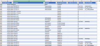
I have a task whereby I have to show;

1. The first date a unique ID failed to login
2. The first time they successfully logged in.
3. The last time they logged in and
4. The amount of times they logged in.

I can do it manually no problem of course but there 639,904 rows and at least 144 unique IDs.

I managed to show the amount of times they logged in using '=SUMPRODUCT(SUBTOTAL(103, OFFSET(D2:D639902, ROW(D2:D639902) - MIN(ROW(D2:D639902)),,1)), --(ISNUMBER(FIND(J1, D2:D639902))))' but I was hoping I could use a formula for each of the results required to make life easier.


EDIT: The formula for the amount of logins doesn't work based in an entry it only works based on my filtering.

 

[JamesCanale]

MrExcelPlayground20 (version 1).xlsb
	A	B	C	D	E	F	G	H	I	J
1	Date	Login	Result
2	12/24/2023	Mary	Fail
3	1/1/2024	Jamie	Fail			Login	First Fail	first Success	Last Login	Logins
4	1/1/2024	Fred	Login			Fred	1/17/2024	1/1/2024	3/20/2024	8
5	1/6/2024	Fred	Login			Jamie	1/1/2024	1/8/2024	2/13/2024	4
6	1/8/2024	Jamie	Login			John		4/10/2024	4/10/2024	1
7	1/9/2024	Mary	ForgotPassword			Mary	12/24/2023	1/15/2024	3/15/2024	5
8	1/11/2024	Jamie	Login			Sally	1/11/2024	4/8/2024	4/8/2024	1
9	1/11/2024	Fred	Login
10	1/11/2024	Sally	Fail
11	1/13/2024	Sally	Timeout
12	1/15/2024	Mary	Login
13	1/17/2024	Fred	Fail
14	1/18/2024	Fred	Login
15	1/30/2024	Mary	Login
16	1/30/2024	Jamie	Login
17	2/2/2024	Fred	Logout
18	2/2/2024	Mary	Login
19	2/13/2024	Jamie	Login
20	2/20/2024	Fred	Logout
21	2/21/2024	Fred	Login
22	2/29/2024	Mary	Login
23	3/3/2024	Jamie	Logout
24	3/8/2024	Fred	Login
25	3/9/2024	Fred	Login
26	3/12/2024	Jamie	Fail
27	3/15/2024	Mary	Login
28	3/18/2024	Jamie	ForgotPassword
29	3/20/2024	Fred	Login
30	4/4/2024	Sally	Timeout
31	4/8/2024	Sally	Login
32	4/9/2024	Mary	ForgotPassword
33	4/10/2024	John	Login
Sheet26

Cell Formulas
Range	Formula
F4:F8	F4	=SORT(UNIQUE(Table1[Login]))
G4:G8	G4	=IFERROR(MIN(FILTER(Table1[Date],(Table1[Login]=F4)*(Table1[Result]="Fail"))),"")
H4:H8	H4	=IFERROR(MIN(FILTER(Table1[Date],(Table1[Login]=F4)*(Table1[Result]="Login"))),"")
I4:I8	I4	=IFERROR(MAX(FILTER(Table1[Date],(Table1[Login]=F4)*(Table1[Result]="Login"))),"")
J4:J8	J4	=IFERROR(ROWS(FILTER(Table1[Date],(Table1[Login]=F4)*(Table1[Result]="Login"))),"")
Dynamic array formulas.

 

[Steve lewis]

Thank you so much, took me a while to work out what you had done but got it in the end. Saved me a lot of monotonous time