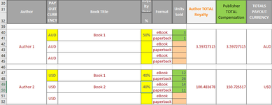
extract values, one from calculated formula

[skunkworks]

In the royalty spreadsheet shown here, authors and their books are listed. Some authors may have only one book, while others may have a dozen. "Author Total Royalty" is a calculated field. I would like to be able to extract the author's name and "Author Total Royalty" into another worksheet. How can this be done?

 

[portews]

Try this:

Sub AuthorInfo()
Dim WkBk As Worksheet
Dim myselect As Range

'set the receiving sheet
Set WkBk = Sheets("Sheet2")
'get the current cell selection
Set myselect = Selection
'stop the screen from showing selection changes
Application.ScreenUpdating = False
'get the last row with data
LastRow1 = Sheets("Sheet1").Range("A" & Rows.Count).End(xlUp).Row
'set the row on the recieving sheet to put the data
j = 2
'select the first cell with data
Cells(34, 1).Select

Do
    'copy the values over to the recieveing sheet
    WkBk.Range("A" & j) = Selection.Value
    WkBk.Range("B" & j) = Selection.Offset(0, 6).Value
    'increment the recieving row
    j = j + 1
    'select the next cell with data
    Selection.End(xlDown).Select
'if the selection row is greater than the last row with data, stop
Loop Until Selection.Row > LastRow1

'set the selection back to original
myselect.Select
'show changes from here
Application.ScreenUpdating = True
End Sub

 

[Alex Blakenburg]

If you don't want to use code, somewhat surprisingly a Pivot Table will get you what you need.

(I thought the Merged Cells would break it but since the 2 fields you interested in being Author and Total Royalty are sized the same and the 1st heading row always contains data it appears to work)

 

[skunkworks]

Try this:

Sub AuthorInfo()
Dim WkBk As Worksheet
Dim myselect As Range

'set the receiving sheet
Set WkBk = Sheets("Sheet2")
'get the current cell selection
Set myselect = Selection
'stop the screen from showing selection changes
Application.ScreenUpdating = False
'get the last row with data
LastRow1 = Sheets("Sheet1").Range("A" & Rows.Count).End(xlUp).Row
'set the row on the recieving sheet to put the data
j = 2
'select the first cell with data
Cells(34, 1).Select

Do
    'copy the values over to the recieveing sheet
    WkBk.Range("A" & j) = Selection.Value
    WkBk.Range("B" & j) = Selection.Offset(0, 6).Value
    'increment the recieving row
    j = j + 1
    'select the next cell with data
    Selection.End(xlDown).Select
'if the selection row is greater than the last row with data, stop
Loop Until Selection.Row > LastRow1

'set the selection back to original
myselect.Select
'show changes from here
Application.ScreenUpdating = True
End Sub

Hi Bill,

Thank you! Disclaimer: I know considerably less than you and am, therefore, much more dangerous.

That said, this is what I did:
Created a new worksheet named Sheet2
1. Pressed Alt+F11 to open the VB window
2. Selected Insert > Module
3. Pasted your code into the module
4. Pressed F5

No results were returned. Where have I gone wrong?

 

[skunkworks]

If you don't want to use code, somewhat surprisingly a Pivot Table will get you what you need.

(I thought the Merged Cells would break it but since the 2 fields you interested in being Author and Total Royalty are sized the same and the 1st heading row always contains data it appears to work)

Thank you, Alex. I tried the range 'Royalty Report Jul-Sep 2022'!B$40:$AD!560 to create a pivot table but received the following message: "Data source reference is not valid." Note that the actual file I'm working with appears to have no column A. I've tried to unhide it with no luck.

 

[portews]

Hi Bill,

Thank you! Disclaimer: I know considerably less than you and am, therefore, much more dangerous.

That said, this is what I did:
Created a new worksheet named Sheet2
1. Pressed Alt+F11 to open the VB window
2. Selected Insert > Module
3. Pasted your code into the module
4. Pressed F5

No results were returned. Where have I gone wrong?

What's the name if the original sheet? If it's not Sheet1, you'll need to replace "Sheet1" with the correct name in the code. You may have to change column numbers if it's not A for the Authors and G for the Author Total Royalty.

You can also use the F8 key to step through the code. Put an apostrophy before the "Application.ScreenUpdating = False" line and you can watch which fields are being selected.

 

[Alex Blakenburg]

Thank you, Alex. I tried the range 'Royalty Report Jul-Sep 2022'!B$40:$AD!560 to create a pivot table but received the following message: "Data source reference is not valid." Note that the actual file I'm working with appears to have no column A. I've tried to unhide it with no luck.

Pivot Tables need to have all columns of the heading row populated. You have not included the heading row in your range. Based on your picture you should have started at row 30 not row 40.
You have not shown your column references, if you have merged columns as well the then pivot tables probably won't work.

Note: the majority of experienced excel users avoid merged cells like the plague. Many functions in excel will not work properly when you have merged cells.

 

[skunkworks]

Pivot Tables need to have all columns of the heading row populated. You have not included the heading row in your range. Based on your picture you should have started at row 30 not row 40.
You have not shown your column references, if you have merged columns as well the then pivot tables probably won't work.

Note: the majority of experienced excel users avoid merged cells like the plague. Many functions in excel will not work properly when you have merged cells.

Alex,

After renaming the worksheet to Sheet1, I used the following to create the pivot table: 'Sheet1'!B$40:$AD!560. It generates the same error. I did not create this spreadsheet, nor do I particularly like it; however, the client does. It is quite complicated, with numerous formulae and an API call to update currency exchange rates. Eek!

 

[Alex Blakenburg]

But did you try 'Sheet1'!B$30:$AD!560.
And I don't know what columns are merged if not all it may help to only include columns from Author to Author Total Royalty

 

[Alex Blakenburg]

If the above doesn't work and you still want to try VBA.
The below assumes: that your output sheet name is called "Sheet2" and that it already exists.
It also assumes that your, total column is "H". If this is not the case then we need to change the range.
Modify the 4 lines that are flagged with "<---"

PS: It also assumes that each Author only appears once in column B. The code will get more complex if this is not the case.

Sub TotalDataMergedCells()

    Dim shtData As Worksheet, shtOut As Worksheet
    Dim rngData As Range, arrData As Variant, arrOut() As Variant
    Dim rngOut As Range
    Dim lrowData As Long, firstrowData As Long, rowOut As Long, i As Long
    Dim totcolData As Long
   
    Set shtData = ActiveSheet
    Set shtOut = Worksheets("Sheet2")               ' <--- Change sheet name to the name of your output sheet
    Set rngOut = shtOut.Range("A1")                 ' <--- Change this to where you want it on the sheet
   
    With shtData
        totcolData = .Columns("H").Column           ' <--- Change to your Royalty Total column
        firstrowData = 30                           ' <--- This needs to be the row where your data starts
        lrowData = .Range("B" & Rows.Count).End(xlUp).Row
        Set rngData = .Range(.Cells(firstrowData, "B"), .Cells(lrowData, totcolData))
    End With
   
    ' Get values
    arrData = rngData.Value
    ReDim arrOut(1 To UBound(arrData, 1), 1 To 2)
    totcolData = totcolData - shtData.Columns("B").Column + 1
    For i = 1 To UBound(arrData)
        If arrData(i, 1) <> "" Then
            rowOut = rowOut + 1
            arrOut(rowOut, 1) = arrData(i, 1)
            arrOut(rowOut, 2) = arrData(i, totcolData)
        End If
    Next i
   
    rngOut.Resize(, 2) = Array("Author", "Royalty Total")   ' Add Headings
    rngOut.Offset(1).Resize(rowOut, 2).Value = arrOut       ' Output Data

End Sub