FALSE return

[toony]

Hi. I have the below formula but not sure how to avoid the FALSE return if you can help please.

=IFERROR(IF(V15="CNY",U15/Y15,IF(V15="USD",U15/Y16)),"")

 

[6StringJazzer]

You are getting a FALSE result because you have this expression in your formula:

IF(V15="USD",U15/Y16)

If V15="USD" you return U15/Y16, but you do not specify a result if V15 is not "USD". Therefore it will return FALSE by default.

Therefore if V15 is not "CNY" and it's not "USD", this formula will return FALSE. What do you want to return in such a case?

Maybe this:

=IFERROR(IF(V15="CNY",U15/Y15,IF(V15="USD",U15/Y16,"")),"")

 

[Peter_SSs]

Another guess

=IFERROR(U15/IF(V15="CNY",Y15,Y16),"")

 

[toony]

Thank you guys for the explanation and the subsequent solution.

I have used =IFERROR(U15/IF(V15="CNY",Y15,Y16),""). I love it because it's short and it works perfect.....but only up to row 16 as attached.

I have also done a much longer formula with an IF statement for each currency but

So, as attached;
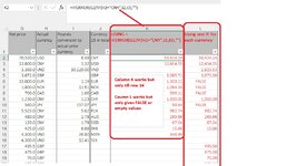
=IFERROR(G2/IF(H2="CNY",I2,I3),"") formula is short and sweet and it works (perfectly) but only up to row 16.

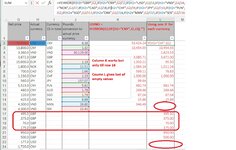
Then, the below is the alternative formula to the above with one IF statement for each currency but, after row 14, only mostly gives empty or FALSE cells;
=IFERROR(IF(H2="GBP",G2,IF(H2="CNY",G2/I2,IF(H2="USD",G2/I3,IF(H2="VND",G2/I4,IF(H2="EUR",IF(G2/I6,IF(H2="NOK",G2/I7,IF(H2="CAD",G2/I8,IF(H2="CHD",G2/I9,IF(H2="JPY",G2/I10,IF(H2="PLN",G2/I11,IF(H2="AUD",G2/I12,IF(H2="SGD",G2/I13,IF(H2="DKK",G2/I14,IF(H2="MXN",G2/I15,IF(H2="SEK",G2/I16)))))))))))))))),"")

 

[toony]

Hi. I have run it again with the long formula. It had a couple of errors in the long formula, but though it doesn't give FALSE anymore,
it gives loads of blank cells, which it should do if it's a GBP currency, but rows 23 and 24 for example are USD and CNY and should give relevant values;
=IFERROR(IF(H2="GBP",G2,IF(H2="CNY",G2/J2,IF(H2="USD",G2/J3,IF(H2="VND",G2/J4,IF(H2="EUR",G2/J6,IF(H2="NOK",G2/J7,IF(H2="CAD",G2/J8,IF(H2="CHF",G2/J9,IF(H2="JPY",G2/J10,IF(H2="PLN",G2/J11,IF(H2="AUD",G2/J12,IF(H2="SGD",G2/J13,IF(H2="DKK",G2/J14,IF(H2="MXN",G2/J15,IF(H2="SEK",G2/J16))))))))))))))),"")

For the shorter below formula, I've tried different ways bust still only gives values up to cell 15 as new document attached;
=IFERROR(G2/IF(H2="CNY",I2,I3),"")

 

[toony]

Apologies, but the long formula I meant to say that it doesn't suppose to give empty cells unless errors.
The GBP correctly gives the same value as in column G.

I have now omitted the IFERRROR so as to see the type of error. Column L only gives DV/0 in row 10, but after column 14 it's DV/0 error in all rows except if the GBP currency which gives whatever value is in column G

 

[rlv01]

Posting screen grabs of your cell data is not very useful, since others cannot easily transfer the data for analysis. You should consider using the xl2BB add in.

tmp1.xlsm
	G	H	I	J	K
1	70,520	USD	8.38	CNY	10454.55
2	13,800	CNY	1.32	USD
Sheet6

Cell Formulas
Range	Formula
K1:K2	K1	=IFERROR(G2/IF(H2="CNY",I2,I3),"")

XL2BB - Excel Range to BBCode

Convert selected range to BBCode to include as a snapshot in your question.

www.mrexcel.com

 

[toony]

Hi Thank you for the advise. Tried to follow it but when i go to browse bottom (3rd bullet) can't see any xl2BB add in

ou need to note where you saved the xl2bb.xlam file then it seems like you have gone astray in this section of the instructions.

 

[toony]

I have tried different way but unable to see/upload it I had to use the Excel Guru forum instead where I can upload an small excel file.
Sorry for the inconvenience. How can i cancel this threat please

 

[jtakw]

Hi,

You're getting FALSE and Blank results with your Long formula because you didn't Anchor column J references in the formula.

This should work.

Put 1 (the number one) in J5 for GBP

Formula in K2, copied down as far as needed:

=IFERROR(G2/LOOKUP(2,1/SEARCH(H2,I$2:I$16),J$2:J$16),"")

MODs will ask, I'm just mentioning it, please provide links to all sites you have Cross-Posted this question.
And you should post a link to this thread at all the sites you've Cross-Posted at.