FALSE return

[toony]

Hi. I have the below formula but not sure how to avoid the FALSE return if you can help please.

=IFERROR(IF(V15="CNY",U15/Y15,IF(V15="USD",U15/Y16)),"")

 

[toony]

Thanks Jtakw. Thanks for the tip. I've used only one site. Link: IF only work up to 16

I did realise that with the long formula i didn't anchor it and it's now working just fine, silly error but not the most experienced. Many thanks.

Regarding the shorter version below, it goes to the bottom now but loads of empty or 0 vaues for somereason.
I have dragged down column L all the way down as indicated. Cheers
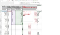
=IFERROR(G2/LOOKUP(2,1/SEARCH(H2,I$2:I$16),J$2:J$16),"")

 

[jtakw]

I have used =IFERROR(U15/IF(V15="CNY",Y15,Y16),""). I love it because it's short and it works perfect.....but only up to row 16 as attached.

You haven't put the 1 (numeric number one) in J5 for GBP as I said in my Post #10 BOLD and Underlined.

Please confirm your table data Starts at I2:I16 for Currency, and J2:J16 for Conversion rate.

Also, just want to point out, the "short" formula in your quote above works ONLY for CNY, as it's the only conditions it checks for, the results you get from that formula will be incorrect.

 

[jtakw]

Again, you MUST put 1 in J5, I put my formula in Column L and it works correctly.
As you can see, All the results in Column K using that other formula are Incorrect, except for K2, the rest are wrong.

Book2.xlsx
	G	H	I	J	K	L
1	Net price	Actual currency	Currency. 15 in total	Pounds conversion to actual price currency	USING = IFERROR(G2/IF(H2="CNY",J2,J3),"")	My Formula
2	70,520.0	USD	CNY	8.38	53,424.24	53424.24242
3	13,800.0	CNY	USD	1.32	10,454.55	1646.778043
4	3,360.0	VND	VND	30,129.00	3,360.00	0.111520462
5	3,672.0	GBP	GBP	1.00	3,085.71	3672
6	15,000.0	EUR	EUR	1.19	1,303.21	12605.04202
7	1,800.0	NOK	NOK	11.51	1,084.34	156.3857515
8	700.0	CAD	CAD	1.66	569.11	421.686747
9	1,230.0	CNY	CHF	1.23	1,000.00	146.778043
10	560.0	JPY	JPY	157.07	99.64	3.565289361
11	5,523.0	CNY	PLN	5.62	982.74	659.0692124
12	480.0	CNY	AUD	1.78	269.66	57.27923628
13	120.0	CNY	SGD	1.79	67.04	14.31980907
14	425.0	USD	DKK	8.88	15.86	321.969697
15	4,300.0	VND	MXN	26.80	346.49	0.142719639
16	4,300.0	VND	SEK	12.41	#DIV/0!	0.142719639
17	495.5	GBP			#DIV/0!	495.5
18	375.0	GBP			#DIV/0!	375
19	70.0	GBP			#DIV/0!	70
20	175.0	GBP			#DIV/0!	175
21	950.0	GBP			#DIV/0!	950
22	500.0	GBP			#DIV/0!	500
23	177.0	USD			#DIV/0!	134.0909091
24	1,720.0	CNY			#DIV/0!	205.2505967
25	14,208.0	CNY			#DIV/0!	1695.465394
Original

Cell Formulas
Range	Formula
K2:K25	K2	=G2/IF(H2="CNY",J2,J3)
L2:L25	L2	=IFERROR(G2/LOOKUP(2,1/SEARCH(H2,I$2:I$16),J$2:J$16),"")

Named Ranges
Name	Refers To	Cells
Currency	=Original!$I$2:$I$16	L2:L25

 

[rlv01]

Hi Thank you for the advise. Tried to follow it but when i go to browse bottom (3rd bullet) can't see any xl2BB add in

ou need to note where you saved the xl2bb.xlam file then it seems like you have gone astray in this section of the instructions.

The file is downloaded as a .zip file. You must extract it into a folder, then browse to find the folder as part of the 3rd bullet point.

 

[toony]

mmmmm. Yes, I thought so, but I think it was giving correct results somehow up to row 14 but yes that's exactly what I thought when I sow it

I sow the below statement but wasn't sure what you meant as obvious as it's now. I've now put there a 1 and it works just fine ;
"You haven't put the 1 (numeric number one) in J5 for GBP as I said in my Post #10 BOLD and Underlined."

And yes, in the screenshot column i is the currency (unique values) and field K is the conversion rate. I just didn't delete the original formula and tried on field L sorry for the confusion

 

[toony]

Yes, I got up to "Browse" but when I browse still can't see the xl2BB add in

 

[jtakw]

Hi,

This should work.

Put 1 (the number one) in J5 for GBP

Formula in K2, copied down as far as needed:

=IFERROR(G2/LOOKUP(2,1/SEARCH(H2,I$2:I$16),J$2:J$16),"")

I sow the below statement but wasn't sure what you meant as obvious as it's now. I've now put there a 1 and it works just fine ;
"You haven't put the 1 (numeric number one) in J5 for GBP as I said in my Post #10 BOLD and Underlined."

And yes, in the screenshot column i is the currency (unique values) and field K is the conversion rate. I just didn't delete the original formula and tried on field L sorry for the confusion

I said you needed to put 1 in J5 in my Post # 10.

So my formula is working for you now ?

 

[jtakw]

Yes, I got up to "Browse" but when I browse still can't see the xl2BB add in

You "Browse" to the folder where you had "Saved" the file during the download.

 

[rlv01]

Yes, I got up to "Browse" but when I browse still can't see the xl2BB add in

A few questions to help clarify.

1. When you clicked on the link to download the file xl2bb.zip, what folder (directory) did you save that to? If you are not sure, then repeat the download and be sure to note the location.
2. When you extracted the add-in file xl2bb.xlam from the compressed downloaded xl2bb.zip file, what folder (directory) did you save xl2bb.xlam to?
3. When you followed the installation instruction and got up to "Browse" did you browse to the folder in item #2 above where your saved copy of xl2bb.xlam is located?

 

[jtakw]

I said you needed to put 1 in J5 in my Post # 10.

So my formula is working for you now ?

A shorter version in M2 copied down:

Book2.xlsx
	G	H	I	J	K	L	M
1	Net price	Actual currency	Currency. 15 in total	Pounds conversion to actual price currency	USING = IFERROR(G2/IF(H2="CNY",J2,J3),"")	My Formula	My Shorter Formula
2	70,520.0	USD	CNY	8.38	53,424.24	53424.24242	53424.24242
3	13,800.0	CNY	USD	1.32	10,454.55	1646.778043	1646.778043
4	3,360.0	VND	VND	30,129.00	3,360.00	0.111520462	0.111520462
5	3,672.0	GBP	GBP	1.00	3,085.71	3672	3672
6	15,000.0	EUR	EUR	1.19	1,303.21	12605.04202	12605.04202
7	1,800.0	NOK	NOK	11.51	1,084.34	156.3857515	156.3857515
8	700.0	CAD	CAD	1.66	569.11	421.686747	421.686747
9	1,230.0	CNY	CHF	1.23	1,000.00	146.778043	146.778043
10	560.0	JPY	JPY	157.07	99.64	3.565289361	3.565289361
11	5,523.0	CNY	PLN	5.62	982.74	659.0692124	659.0692124
12	480.0	CNY	AUD	1.78	269.66	57.27923628	57.27923628
13	120.0	CNY	SGD	1.79	67.04	14.31980907	14.31980907
14	425.0	USD	DKK	8.88	15.86	321.969697	321.969697
15	4,300.0	VND	MXN	26.80	346.49	0.142719639	0.142719639
16	4,300.0	VND	SEK	12.41	#DIV/0!	0.142719639	0.142719639
17	495.5	GBP			#DIV/0!	495.5	495.5
18	375.0	GBP			#DIV/0!	375	375
19	70.0	GBP			#DIV/0!	70	70
20	175.0	GBP			#DIV/0!	175	175
21	950.0	GBP			#DIV/0!	950	950
22	500.0	GBP			#DIV/0!	500	500
23	177.0	USD			#DIV/0!	134.0909091	134.0909091
24	1,720.0	CNY			#DIV/0!	205.2505967	205.2505967
25	14,208.0	CNY			#DIV/0!	1695.465394	1695.465394
Original

Cell Formulas
Range	Formula
K2:K25	K2	=G2/IF(H2="CNY",J2,J3)
L2:L25	L2	=IFERROR(G2/LOOKUP(2,1/SEARCH(H2,I$2:I$16),J$2:J$16),"")
M2:M25	M2	=IFERROR(G2/VLOOKUP(H2,I$2:J$16,2,0),"")

Named Ranges
Name	Refers To	Cells
Currency	=Original!$I$2:$I$16	L2:M25