Filters Problem

jhncloud

New Member
Joined
Dec 7, 2021
Messages
8
Office Version
  1. 2019
Platform
  1. Windows
Hi,

I was wondering if anyone can help. I want a filter sort out table on one sheet to a breakdown on another sheet.

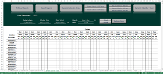
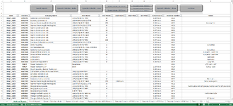
To explain, I have two sheets. Sheet1 is Archived Reports. Sheet2 is a "Dynamic" Calendar. I need both of them to somehow connect in a very specific way. On Sheet2, I need to show on Invoice Numbers Column from a specific date range. On Sheet2, I currently have =FILTER(Table2[Invoice '#],(Table2[Machine Number]=H5)*(Table2[Date]=O8),"Not Found") on B16, it works for just one date which is cell O8, but I need it to show the invoice number for multiple dates.

I'm not sure what formula to use to achieve that.

Thanks for the help.
John S.
 

Attachments

  • Screenshot 2023-11-13 151414.png
    Screenshot 2023-11-13 151414.png
    112.8 KB · Views: 10
  • Screenshot 2023-11-13 151400.png
    Screenshot 2023-11-13 151400.png
    180.2 KB · Views: 10

Excel Facts

Format cells as date
Select range and press Ctrl+Shift+3 to format cells as date. (Shift 3 is the # sign which sort of looks like a small calendar).
It's not clear to me what you mean by "show the invoice number for multiple dates". Do you mean that you'd like to specify a start and end date and include any invoices between those dates?...or do you want to specify multiple, discrete dates and include invoices falling on those dates? I've assumed you want the former (see example below). I also notice that the same invoice number appears multiple times. Should each occurrence be displayed, or do you want to see only unique invoice numbers?
MrExcel_20231113.xlsx
BHNO
4Machine #
56032
6
7Date
8Begin5/1/2023
9End5/2/2023
10
11
12
13
14
15Invoice #
1660411797
1760411770
1860411707
1960411707
2060411783
2160411783
2260411783
2360411783
2460411783
2560411783
2660411818
2760411941
2860411941
2960411979
3060411707
3160411707
3260411877
3360411877
3460411877
3560411927
3660411927
Sheet2
Cell Formulas
RangeFormula
B16:B36B16=FILTER(Table2[Invoice '#],(Table2[Machine Number]=H5)*(Table2[Date]>=O8)*(Table2[Date]<=O9),"Not Found")
Dynamic array formulas.
 
Upvote 0
Sorry for the confusion. I was just wondering if I can place a formula on B15 to grab the Invoice# from the Reports Sheet with two conditions: it will filter and grab invoice numbers with the machine # and with the date range on Row 14. I think I should also mention that there are two buttons on ranges AD6:AH7 which subtracts 7 days from S7 and AI6:AI7 which adds 7 days to S7. The machine# is on H4.

Laser - Material Processing.xlsm
ABCDEFGHIJK
1
2DateInvoice #Company NameItem Name# of PiecesLead HoursStart TimeEnd TimeActual HoursMachine NumberNotes
3May 1, 202360411797Carbonex Contractors Ltd..375 (3/8) HR PLT 44W101.00 hours6032
4May 1, 202360411770Economy Conrete Ltd..135 HR SHT A1011 CS TP B561.00 hours6032
5May 1, 202360411707Kaymor Machining & Welding Ltd..188 (3/16) HR PLT 44W2500.50 hours6032Incomplete
6May 1, 202360411707Kaymor Machining & Welding Ltd..135 HR SHT A1011 CS TP B500.50 hours6032
7May 1, 202360411783Kaynic Construction Ltd..750 (3/4) HR PLT 44W30.67 hours6032
8May 1, 202360411783Kaynic Construction Ltd..500 (1/2) HR PLT 44W160.67 hours6032
9May 1, 202360411783Kaynic Construction Ltd..313 (5/16) HR PLT 44W40.67 hours6032
10May 1, 202360411783Kaynic Construction Ltd..188 (3/16) HR PLT 44W200.67 hours6032
11May 1, 202360411783Kaynic Construction Ltd..250 (1/4) HR PLT 44W60.67 hours6032
12May 1, 202360411783Kaynic Construction Ltd..375 (3/8) HR PLT 44W1480.67 hours6032
13May 1, 202360411818Sundown Oilfield Services Ltd..120 HR SHT A1011 CS TP B10.20 hours6032
14May 2, 202360411941All Class Fabrication Ltd..250 (1/4) HR PLT 44W20.20 hours6032
15May 2, 202360411941All Class Fabrication Ltd..375 (3/8) HR PLT 44W40.20 hours6032
16May 2, 202360411979Carbonex Contractors Ltd..375 (3/8) HR PLT 44W320.40 hours6032No issues
17May 2, 202360411707Kaymor Machining & Welding Ltd..188 (3/16) HR PLT 44W2502.00 hours1.50 hours6032Recut some parts
18May 2, 202360411707Kaymor Machining & Welding Ltd..135 HR SHT A1011 CS TP B501.50 hours6032
19May 2, 202360411877Murphy Group Canada.375 (3/8) HR PLT 44W20.50 hours6032Had trouble with 3/4 pieces, had to wait for 3/4 50w to be cut
20May 2, 202360411877Murphy Group Canada.750 (3/4) HR PLT 400F40.50 hours6032
21May 2, 202360411877Murphy Group Canada1 HR PLT 50W10.50 hours6032
22May 2, 202360411927Paragon Oilfield Supply LP..625 (5/8) HR PLT 44W LQ10.60 hours6032Had to recut 5/8
23May 2, 202360411927Paragon Oilfield Supply LP..500 (1/2) HR PLT 44W30.60 hours6032
24May 2, 202360411927Paragon Oilfield Supply LP..375 (3/8) HR PLT 44W10.20 hours60321/2 rip cut
25May 2, 202360411593Rheton Welding Services Ltd..141 STLS TP604L 2B304.00 hours6032SS/Problems with nitro over 33
26May 2, 202360411725Therrien Welding.125 ALUM SHT 5052-H32 SPV10.40 hours6032Aluminum (Cash Sale)
27May 4, 202360411968Torque Industrial Ltd..060 HR SHTT A1011 CS TP B110.50 hours0.10 hours6032
28May 4, 202360411968Torque Industrial Ltd..188 (3/16) HR PLT 44W11.00 hours0.10 hours6032
29May 4, 202360411968Torque Industrial Ltd..250 (1/4) HR PLT 44W10.10 hours6032
30May 4, 202360411968Torque Industrial Ltd..375 (3/8) HR PLT 44W912.00 hours0.10 hours6032
31May 10, 202360412117Alloy Industries.188 (3/16) HR PLT 44W11.00 hours0.30 hours6032
32May 10, 202360412199Alloy Industries.500 (1/2) HR PLT 44W61.00 hours0.60 hours6032
33May 10, 202360412090Kaymor Machining & Welding Ltd.1 HR PLT 44W10.60 hours0.13 hours6032
34May 10, 202360412200Kaymor Machining & Welding Ltd..250 (1/4) HR PLT 44W81.10 hours0.13 hours6032
35May 10, 202360412200Kaymor Machining & Welding Ltd..313 (5/16) HR PLT 44W80.13 hours6032
36May 10, 202360412322Kaymor Machining & Welding Ltd..250 (1/4) HR PLT 44W11.20 hours0.50 hours6032
37May 10, 202360412423Kaynic Construction Ltd..750 (3/4) HP PLT 44W10.40 hours1.00 hours6032
38May 10, 202360412035Roger's Repair & Welding Ltd..120 HR SHT A1011 CS TP B1742.00 hours1.00 hours6032
Report


Laser - Material Processing.xlsm
ABCDEFGHIJKLMNOPQRSTUVWXYZAAABACADAEAFAGAHAIAJAKALAMANAOAPAQARASATAUAVAW
3
4Fixed Parameters6032
5
6Today's DateModay DateDate SelectMonthNovember11
711/13/20235/1/20235/1/2023-196Year2023
8
9
10Dates
11MayMayMayMayMayMayMayMayMayMayMayMayMayMayMayMayMayMayMayMayMayMayMay
12Invoice NumbersMonTueWedThuFriSatSunMonTueWedThuFriSatSunMonTueWedThuFriSatSunMonTue
13AMPMAMPMAMPMAMPMAMPMAMPMAMPMAMPMAMPMAMPMAMPMAMPMAMPMAMPMAMPMAMPMAMPMAMPMAMPMAMPMAMPMAMPMAMPM
1401010202030304040505060607070808090910101111121213131414151516161717181819192020212122222323
1560411797
1660411770
1760411707
1860411707
1960411783
2060411783
2160411783
2260411783
2360411783
2460411783
2560411818
26
27
28
Monthly
Cell Formulas
RangeFormula
AB6AB6=VLOOKUP(W6,'C:\Users\josanche\Desktop\[Master Records - Material Processing.xlsm]Fixed Data'!C4:D15,2,0)
D7D7=TODAY()
J7J7=C14
O7O7=D7+S7
C11,E11,G11,I11,K11,M11,O11,Q11,S11,U11,W11,Y11,AA11,AC11,AE11,AG11,AI11,AK11,AM11,AO11,AQ11,AS11,AU11C11=C14
C12,E12,G12,I12,K12,M12,O12,Q12,S12,U12,W12,Y12,AA12,AC12,AE12,AG12,AI12,AK12,AM12,AO12,AQ12,AS12,AU12C12=C14
C14C14=O7-(IF(WEEKDAY(O7)=1,6,(WEEKDAY(O7)-2)))
D14,F14,H14,J14,L14,N14,P14,R14,T14,V14,X14,Z14,AB14,AD14,AF14,AH14,AJ14,AL14,AN14,AP14,AR14,AT14,AV14D14=C14
E14,G14,I14,K14,M14,O14,Q14,S14,U14,W14,Y14,AA14,AC14,AE14,AG14,AI14,AK14,AM14,AO14,AQ14,AS14,AU14E14=D14+1
B15:B25B15=FILTER(Table2[Invoice '#],Table2[Date]=$C$14,"Not Found")
Dynamic array formulas.
Cells with Data Validation
CellAllowCriteria
W6:AA6List=Month
W7:AA7List=Years


Thanks,
John S.
 
Upvote 0
Have you examined my suggestion in post #2? Adapted to what I believe is the intended start date and end date for your query, it would look like the example below, where the first and last date cells in row 14 are used. I don't understand the significance of adding or subtracting 7 days with the AD6:AH7 and AI6:AI7 buttons. I'm assuming the fixed cell positions C14 and AV14 establish the date range that should be used for the query. As a side note, I would strongly advise against using merged cells in the worksheet, especially where formulas are involved. If this is done as a convenient way to center text across multiple columns, consider instead unmerging the cells and then select the cells that were previously merged and then Home>Alignment and format with "Center Across Selection". This achieves the same appearance.
MrExcel_20231113.xlsx
BCDEF
11MayMay
12Invoice NumbersMonTue
13AMPMAMPM
1401010202
1560411797
1660411770
1760411707
1860411707
1960411783
Monthly
Cell Formulas
RangeFormula
C11,E11C11=C14
C12,E12C12=C14
C14C14=O7-(IF(WEEKDAY(O7)=1,6,(WEEKDAY(O7)-2)))
D14,F14D14=C14
E14E14=D14+1
B15:B50B15=FILTER(Table2[Invoice '#],(Table2[Machine Number]=H4)*(Table2[Date]>=C14)*(Table2[Date]<=AV14),"Not Found")
Dynamic array formulas.

Also, please update your profile to show your Excel version. You've indicated use of the FILTER function, so Excel 2019 must not be the current version in use.
 
Upvote 0
Assuming you have Excel 365, here is a small sample showing an easier way to form the Monthly output table that relies on formulas that "spill". The approach here reimagines how to form the upper table rows, and rather than use cell C14 to compute the 1st Monday date of interest, that is handled instead by cell J7. Then all dates in the table reference J7 to establish the 46-cell (23 days) calendar. To take advantage of this feature, the cells will need to be unmerged. Then the formula is placed in the first cell of its intended range and the results will automatically spill, much like what you had originally with the FILTER formula.
MrExcel_20231113.xlsx
BCDEFGHIJKLMNOPQRST
3
4Fixed Parameters6032
5
6Today's DateMonday DateDate Select
711/14/20235/1/20235/2/2023-196
8
9
10Dates
11MayMayMayMayMayMayMayMayMayMayMayMayMayMayMayMayMayMay
12Invoice NumbersMonMonTueTueWedWedThuThuFriFriSatSatSunSunMonMonTueTue
13AMPMAMPMAMPMAMPMAMPMAMPMAMPMAMPMAMPM
14010102020303040405050606070708080909
1560411797
1660411770
1760411707
1860411707
1960411783
Monthly
Cell Formulas
RangeFormula
D7D7=TODAY()
J7J7=O7-(IF(WEEKDAY(O7)=1,6,(WEEKDAY(O7)-2)))
O7O7=D7+S7
C11:AV11C11=C14#
C12:AV12C12=C14#
C13:AV13C13=LET(s,SEQUENCE(1,46),IF(ISODD(s),"AM","PM"))
C14:AV14C14=J7+FLOOR(SEQUENCE(1,46,0,0.5),1)
B15:B50B15=FILTER(Table2[Invoice '#],(Table2[Machine Number]=H4)*(Table2[Date]>=C14)*(Table2[Date]<=AV14),"Not Found")
Dynamic array formulas.
 
Upvote 0
Solution
Assuming you have Excel 365, here is a small sample showing an easier way to form the Monthly output table that relies on formulas that "spill". The approach here reimagines how to form the upper table rows, and rather than use cell C14 to compute the 1st Monday date of interest, that is handled instead by cell J7. Then all dates in the table reference J7 to establish the 46-cell (23 days) calendar. To take advantage of this feature, the cells will need to be unmerged. Then the formula is placed in the first cell of its intended range and the results will automatically spill, much like what you had originally with the FILTER formula.
MrExcel_20231113.xlsx
BCDEFGHIJKLMNOPQRST
3
4Fixed Parameters6032
5
6Today's DateMonday DateDate Select
711/14/20235/1/20235/2/2023-196
8
9
10Dates
11MayMayMayMayMayMayMayMayMayMayMayMayMayMayMayMayMayMay
12Invoice NumbersMonMonTueTueWedWedThuThuFriFriSatSatSunSunMonMonTueTue
13AMPMAMPMAMPMAMPMAMPMAMPMAMPMAMPMAMPM
14010102020303040405050606070708080909
1560411797
1660411770
1760411707
1860411707
1960411783
Monthly
Cell Formulas
RangeFormula
D7D7=TODAY()
J7J7=O7-(IF(WEEKDAY(O7)=1,6,(WEEKDAY(O7)-2)))
O7O7=D7+S7
C11:AV11C11=C14#
C12:AV12C12=C14#
C13:AV13C13=LET(s,SEQUENCE(1,46),IF(ISODD(s),"AM","PM"))
C14:AV14C14=J7+FLOOR(SEQUENCE(1,46,0,0.5),1)
B15:B50B15=FILTER(Table2[Invoice '#],(Table2[Machine Number]=H4)*(Table2[Date]>=C14)*(Table2[Date]<=AV14),"Not Found")
Dynamic array formulas.

Thanks for the clarification, I just realized that I was doing it the hard when there was a work around to my problem.
 
Upvote 0

Forum statistics

Threads
1,215,091
Messages
6,123,062
Members
449,089
Latest member
ikke

We've detected that you are using an adblocker.

We have a great community of people providing Excel help here, but the hosting costs are enormous. You can help keep this site running by allowing ads on MrExcel.com.
Allow Ads at MrExcel

Which adblocker are you using?

Disable AdBlock

Follow these easy steps to disable AdBlock

1)Click on the icon in the browser’s toolbar.
2)Click on the icon in the browser’s toolbar.
2)Click on the "Pause on this site" option.
Go back

Disable AdBlock Plus

Follow these easy steps to disable AdBlock Plus

1)Click on the icon in the browser’s toolbar.
2)Click on the toggle to disable it for "mrexcel.com".
Go back

Disable uBlock Origin

Follow these easy steps to disable uBlock Origin

1)Click on the icon in the browser’s toolbar.
2)Click on the "Power" button.
3)Click on the "Refresh" button.
Go back

Disable uBlock

Follow these easy steps to disable uBlock

1)Click on the icon in the browser’s toolbar.
2)Click on the "Power" button.
3)Click on the "Refresh" button.
Go back
Back
Top