bmsmith311
New Member
- Joined
- May 1, 2022
- Messages
- 12
- Office Version
- 2019
- Platform
- MacOS
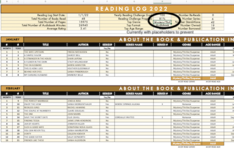
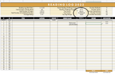
Hi there! I made a spreadsheet and I'm trying to have it autocalculate data, but I'm looking to find the most often recurring text values. This spreadsheet is broken down by month and I'm trying to have one box give a "running total" for the year as the user fills in the data, but obviously we aren't going to have any data for the later months until later in the year so without placeholders, it'll throw an error code. Here is what I currently have:
where the I column is showing a particular genre of a book that a person read. For this formula, as I understand it, I can't skip cells or select only certain ranges within the same column, so while it will ignore zero or blank, it's also including each month's totals (which will be errors until those months are filled in) and I think that's what's causing the error for my "grand total" cell.
Is there a way to skip cells that show an error? I tried a few things after a google search but none of them seemed to work.
Thank you!
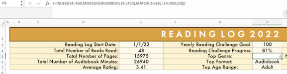
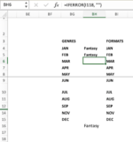
Excel Formula:
=INDEX(I14:I450,MODE(IF(I14:I450<>"",MATCH(I14:I450,I14:I450,0))))Is there a way to skip cells that show an error? I tried a few things after a google search but none of them seemed to work.
Thank you!