I see, so you actually want to "colour" or actually Highlight the cells, rather than change data inside (sorry, I missed that from your original post). As far as I know there's no formula as such to achieve what you need, sorry.
Closest I I would suggest perhaps a TOTAL US and TOTAL THEM cell be added at the bottom of your list, with a COUNTA to give a total. Then conditional format each total based on the other.
Not really what you want to achieve .. but some kind of highlight
| Book1 |
|---|
|
|---|
| J | K | L |
|---|
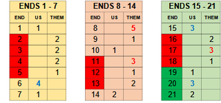
| 1 | ENDS 15 - 21 | | |
|---|
| 2 | | | |
|---|
| 3 | END | lJS | THEM |
|---|
| 4 | 15 | 3 | |
|---|
| 5 | 16 | | 2 |
|---|
| 6 | 17 | | 3 |
|---|
| 7 | 18 | | 1 |
|---|
| 8 | 19 | 1 | |
|---|
| 9 | 20 | 3 | |
|---|
| 10 | 21 | 2 | |
|---|
| 11 | | | |
|---|
| 12 | | TOTAL | TOTAL |
|---|
| 13 | | 4 | 3 |
|---|
| 14 | | | |
|---|
|
|---|