Formula to count how many different days someone worked

[luckeyjune]

Hello,
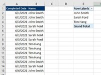
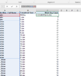
I'm stumped on this seemingly simple request. Basically I have a dataset with a column for name, another for job #, and another for date. Each name has multiple rows with the same date, since there are multiple jobs for day. I want a sum of unique dates each person worked for the month so far. Basically just a sum of worked days. Suggestions for going about this in an easy way? I figured I'd make a pivot of unique names, and do a vlookup helper column next to the pivot of unique names with a count of their workdays. Thanks so much for any and all suggestions!!

 

[JamesCanale]

MrExcelPlayground2.xlsm
	J	K	L	M	N
1	Date	Person	Date Range
2	6/2/2021	John	6/1/2021	John	2
3	6/2/2021	John	6/30/2021	Mary	3
4	6/6/2021	John		Fred	2
5	6/2/2021	Mary
6	6/2/2021	Mary
7	6/3/2021	Mary
8	6/4/2021	Mary
9	6/1/2021	Fred
10	6/1/2021	Fred
11	6/2/2021	Fred
Sheet36

Cell Formulas
Range	Formula
N2:N4	N2	=SUM(--NOT(ISNA(VLOOKUP(ROW(INDIRECT($L$2&":"&$L$3)),IF($K$2:$K$11=M2,$J$2:$J$11,""),1,FALSE))))

 

[luckeyjune]

MrExcelPlayground2.xlsm
	J	K	L	M	N
1	Date	Person	Date Range
2	6/2/2021	John	6/1/2021	John	2
3	6/2/2021	John	6/30/2021	Mary	3
4	6/6/2021	John		Fred	2
5	6/2/2021	Mary
6	6/2/2021	Mary
7	6/3/2021	Mary
8	6/4/2021	Mary
9	6/1/2021	Fred
10	6/1/2021	Fred
11	6/2/2021	Fred
Sheet36

Cell Formulas
Range	Formula
N2:N4	N2	=SUM(--NOT(ISNA(VLOOKUP(ROW(INDIRECT($L$2&":"&$L$3)),IF($K$2:$K$11=M2,$J$2:$J$11,""),1,FALSE))))

Thank you so much for your reply. When I try to implement this in my actual sheet, it's not working.. I think this might be due to the date field in the original dataset not being formatted as a date. It would be nice to find a way that doesn't require the date range, and can somehow just count unique values by name.

 

[JamesCanale]

I added a bunch of helper columns (2 for each person). It allows you to ignore the date range. You can ignore columns L and N here.

MrExcelPlayground2.xlsm
	J	K	L	M	N	O	P	Q	R	S	T	U
1	Date	Person	Date Range				Helper Columns for each person
2	6/2/2021	John	6/1/2021	John	2	2	44349			44349	44349	44348
3	6/2/2021	John	6/30/2021	Mary	3	3	44349			44353	44350	44349
4	6/6/2021	John		Fred	2	2	44353				44351
5	6/2/2021	Mary						44349
6	6/2/2021	Mary						44349
7	6/3/2021	Mary						44350
8	6/4/2021	Mary						44351
9	6/1/2021	Fred							44348
10	6/1/2021	Fred							44348
11	6/2/2021	Fred							44349
Sheet36

Cell Formulas
Range	Formula
N2:N4	N2	=SUM(--NOT(ISNA(VLOOKUP(ROW(INDIRECT($L$2&":"&$L$3)),IF($K$2:$K$11=M2,$J$2:$J$11,""),1,FALSE))))
O2	O2	=COUNT(S2:S11)
P2:P11	P2	=IF(K2:K11=M2,J2:J11,"")
Q2:Q11	Q2	=IF(K2:K11=M3,J2:J11,"")
R2:R11	R2	=IF(K2:K11=M4,J2:J11,"")
S2:U11	S2	=IFERROR(INDEX(P$2#,MATCH(0,INDEX(COUNTIF(S$1:S1,P$2#),0,0),0)),"")
O3	O3	=COUNT(T2:T11)
O4	O4	=COUNT(U2:U11)
Dynamic array formulas.

Excel 365s "UNIQUE" function would make quick work of this.

Other clever folk on here might be able to do this more elegantly.

 

[Fluff]

Another option

+Fluff 1.xlsm
	A	B	C	D	E
1	Date	Person
2	02/06/2021	John		John	2
3	02/06/2021	John		Mary	3
4	06/06/2021	John		Fred	2
5	02/06/2021	Mary
6	02/06/2021	Mary
7	03/06/2021	Mary
8	04/06/2021	Mary
9	01/06/2021	Fred
10	01/06/2021	Fred
11	02/06/2021	Fred
12
List

Cell Formulas
Range	Formula
E2:E4	E2	=SUM(--(FREQUENCY(IF($B$2:$B$11=D2,$A$2:$A$11),$A$2:$A$11)>0))
Press CTRL+SHIFT+ENTER to enter array formulas.

 

[luckeyjune]

Thank you so much for these interesting solutions! Because in my original dataset I have so many names and dates, after attempting the options presented here I decided to do a pivot on another tab, with a column for name, and another for date. I made it so the pivot repeats the column label for name on each line to enable the ability to vlookup. I put a helper column to the right of the pivot and use COUNTIF to count how many times the name appears, which will in turn count the unique dates, since the pivot only shows unique dates. Then in my original data I did a VLOOKUP for name, and pulled in the day #. That way I can pivot the entire dataset. Maybe not that elegant, but I think this is the easiest for me to maintain when running this report weekly. Thank you everyone for your help. I learn a LOT from this site.

 

[Fluff]

Glad you sorted it & thanks for the feedback.

 

[luckeyjune]

Glad you sorted it & thanks for the feedback.

Thank you so much. I am going to save your formula idea in my little catalogue of formulas I keep in notepad though. I am sure I'll find it useful. Thanks again - this site is always enlightening.