Hello Nicola,
I have the following codes which I believe will do the task for you.
Firstly, place this code into the worksheet module (your input sheet):
VBA Code:
Private Sub Worksheet_SelectionChange(ByVal Target As Range)

        If Target.Cells.Count > 1 Then Exit Sub

    Application.ScreenUpdating = False
    Application.EnableEvents = False

        If Target.Column = 1 And Target.Row > 4 And Target.Value <> vbNullString Then
              Target.Offset(, 1).Value = Now
              Target.Offset(, 2).Value = Now + TimeSerial(Me.[C1].Value, 0, 0) 'Adds selected hours from the cell C1 dropdown to the estimated return time in the relevant cell in Column B.
              Target.Offset(, 1).Interior.ColorIndex = 3
        End If

        If Target.Column = 9 And Target.Row > 4 Then
              If Target.Offset(, -7) <> "" Then
                    Target.Value = Now
                    Target.Interior.ColorIndex = 4
              End If
        End If

    Me.Columns.AutoFit
    Application.EnableEvents = True
    Application.ScreenUpdating = True

End Sub
To implement this code:-
-Right click on the sheet tab.
- Select "View Code" from the menu that appears.
- In the big white code field that then appears, paste the above code.
What this code does:-
- When a User clicks on their name in Column A, a date/time stamp will appear in Column B adjacent to their name. On the same row, in Column C, the same date/time stamp will appear. However, as you need an estimated return time in this column, the User can select a number from a drop down list in cell C1. These numbers represent hours. So, if the expected return time is in an hour's time, the user needs to select the number 1 from the list (and so on). This selection will increment the time in the date stamp.
Please note that the User will need to select from the drop down prior to clicking on their name. This will save the User having to manually attempt to place an estimated time in the cell.
- When a User returns, all they need to do is to click on the relevant cell (on the same row as their name) in Column I (the "Returned" column). Another date/time stamp will appear showing their logged back in time.
Next, place the two following codes into a standard module:-
VBA Code:
Sub TestMail()

    Dim c As Range, Rng As Range, sh As Worksheet
    Set sh = Sheet1
    Set Rng = sh.Range("J3", sh.Range("J" & sh.Rows.Count).End(xlUp))

    Application.ScreenUpdating = False

             With Rng
                    .AutoFilter 1, "Late"
                    .Offset(1, -9).Copy Sheet1.[M1]
                    .AutoFilter
             End With
                    SendMail

    sh.Columns(13).Clear
    sh.Columns.AutoFit
    Application.ScreenUpdating = True

End Sub
Sub SendMail()

    Dim oApp As Object, oMail As Object, MailBody As String
    Dim sh As Worksheet

    Set sh = Sheet1
    Set oApp = CreateObject("Outlook.Application")
    Set oMail = oApp.CreateItem(0)

Application.ScreenUpdating = False

                MailBody = "Please be advised that " & sh.Range("B1").Value & " returned later than estimated." & vbNewLine & _
                           "Please check."
                On Error Resume Next
                  With oMail
                      .To = "YOUR EMAIL ADDRESS HERE"
                      .CC = ""
                      .BCC = ""
                      .Subject = "Re:" & sh.Range("B1").Value
                      .Body = MailBody
                      .Send
                  End With

    MsgBox "Message sent to the Head Honcho.", vbExclamation, "ADVICE"
    Set oMail = Nothing
    Set oApp = Nothing

Application.ScreenUpdating = True

End Sub
Assign
ONLY the "TestMail" code to a button on your input sheet. This code will call the "SendMail" code.
On the input sheet, you'll require another column, Column J and title it, say, "Status".
On the input sheet, place this formula in Column J starting in C5 and dragging it down as far as needed:-
=IF(AND(NOW()>C5,C5<>""),"Late","")
This formula will determine which Users have returned later than the estimated return time. From here, once the "Email" button is clicked on, the code will filter for "Late" and send the details of all late returning Users to the email address you specify in the code (see "YOUR EMAIL ADDRESS HERE" in the code). Please ensure that the formula is not interfered with.
Also, in cell B1 of the input sheet, there is another formula:
=TEXTJOIN(", ",,M1:M50)
This formula simply concatenates all the names of the late-returning Users, after their names are filtered and placed temporarily in Column M, and added to the email sent to the specified email address. Cell B1 simply stores the names and bundles them off in the one email.
Test all this in a copy of your workbook first.
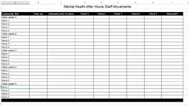
I've added a mock-up workbook for you
here. Click on some User names then select ,say, the number 1 from the drop down in C1, then click on a couple of more user names. You'll note those designated as "Late" in Column J. Click on the "Email" button, then check your emails.
Don't forget to add your email address to the code.
I hope that this helps.
Cheerio,
vcoolio.