Help with complicated formula

Todd Kolar

New Member
Joined
Feb 7, 2024
Messages
10
Office Version
  1. 2016
Platform
  1. Windows
I'm a pretty avid Excel formula writer, however, I cannot figure out how to make this particular challenge work.
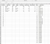
Attached is a screenshot of what I'm trying to accomplish.
I have a list of names in column B that have to repeat in several rows in Column I.
The rows needed are shown in column G which shows how many times the name needs to repeat.
For instance names "R15,109" and "XX,2" need only one instance so they are in order in column I as 1 and 2.
However, name "R15,111-118" needs 8 instances or rows so they are in order in column I as 3-10.
Then name "xx,19-36" needs 2 instances or rows in column I so it is at 10-11.
And you can see the pattern and the rest of the names how they need to be ordered.
The sum of the rows needed in column G total the number of rows in column H based on how many times the name needs to repeat.
Column I is where I need the formula to work and I just typed in the names for reference.
I'm at my wits end so I greatly appreciate any help on solving this one and I hope my explanation makes sense.
Thanks for reading this!

T
 

Attachments

  • Excel Help.JPG
    Excel Help.JPG
    125.5 KB · Views: 10

Excel Facts

What is the fastest way to copy a formula?
If A2:A50000 contain data. Enter a formula in B2. Select B2. Double-click the Fill Handle and Excel will shoot the formula down to B50000.
For 2016, I think I'd add a running total column next to column G, then you could fill your row number sequence down and use an INDEX/MATCH to get the right list name. Well, I'd use Power Query, but you said you wanted a formula. ;)
 
Upvote 0
I2, copied down:

=IFERROR(INDEX($B$2:$B$6,MATCH(0,INDEX(--(COUNTIF($I$1:I1,$B$2:$B$6)=$G$2:$G$6),0),0)),"")
 
Upvote 0
My description was very bad, so here is an example of what I was trying to suggest!

Book3
ABCDEFGHIJ
1List OrderList NamePrefixRange1st NumberLast NumberRows neededRTRowsFinal Name
21R15, 109R15109109109111R15, 109
32XX,2XX222122XX,2
43R15, 111-118R16111-118111118833R15, 111-118
54XX,11-12XX11-1211122114R15, 111-118
65R15,121-126R17121-1261211266135R15, 111-118
76XX,19-36XX19-36193618196R15, 111-118
877R15, 111-118
988R15, 111-118
1099R15, 111-118
111010R15, 111-118
121111XX,11-12
131212XX,11-12
141313R15,121-126
151414R15,121-126
161515R15,121-126
171616R15,121-126
181717R15,121-126
191818R15,121-126
201919XX,19-36
212020XX,19-36
2221XX,19-36
2322XX,19-36
2423XX,19-36
2524XX,19-36
2625XX,19-36
2726XX,19-36
2827XX,19-36
2928XX,19-36
3029XX,19-36
3130XX,19-36
3231XX,19-36
3332XX,19-36
3433XX,19-36
3534XX,19-36
3635XX,19-36
3736XX,19-36
3837 
3938 
4039 
4140 
4241 
Sheet1
Cell Formulas
RangeFormula
G2:G7G2=F2-E2+1
H2:H7H2=SUM(G$1:G1)+1
J2:J42J2=IF(I2>SUM($G$2:$G$7),"",INDEX($B$2:$B$7,MATCH(I2,$H$2:$H$7,1)))
 
Upvote 0
I2, copied down:

=IFERROR(INDEX($B$2:$B$6,MATCH(0,INDEX(--(COUNTIF($I$1:I1,$B$2:$B$6)=$G$2:$G$6),0),0)),"")
Wow!!! That worked like a charrm!!!! I never could understand the proper use of index with match so thank you soooooooooo very much! You are a lifesaver!
 
Upvote 0
My description was very bad, so here is an example of what I was trying to suggest!

Thank you for the feedback as I will definitely use this in future formulas!
 
Last edited by a moderator:
Upvote 0

Forum statistics

Threads
1,215,069
Messages
6,122,959
Members
449,096
Latest member
Anshu121

We've detected that you are using an adblocker.

We have a great community of people providing Excel help here, but the hosting costs are enormous. You can help keep this site running by allowing ads on MrExcel.com.
Allow Ads at MrExcel

Which adblocker are you using?

Disable AdBlock

Follow these easy steps to disable AdBlock

1)Click on the icon in the browser’s toolbar.
2)Click on the icon in the browser’s toolbar.
2)Click on the "Pause on this site" option.
Go back

Disable AdBlock Plus

Follow these easy steps to disable AdBlock Plus

1)Click on the icon in the browser’s toolbar.
2)Click on the toggle to disable it for "mrexcel.com".
Go back

Disable uBlock Origin

Follow these easy steps to disable uBlock Origin

1)Click on the icon in the browser’s toolbar.
2)Click on the "Power" button.
3)Click on the "Refresh" button.
Go back

Disable uBlock

Follow these easy steps to disable uBlock

1)Click on the icon in the browser’s toolbar.
2)Click on the "Power" button.
3)Click on the "Refresh" button.
Go back
Back
Top