Help with improving formula

[GA036872]

Hi everyone

I copied the following code from a YouTube tutorial:

The code does as instructed but the workbook is very slow and sometimes crashes. I am using =XLOOKUP formula to retrieve data from another workbook called Mail Merge Data to return a customer's name, address, suburb, and postcode. Can anyone advise how this can be improved/simplified so that the workbook isn't so slow?

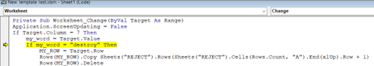
Occasionally, we need to paste "DESTROY" not "destroy" in the override column, but I haven't been able to work out how to get VBA to ignore whether the text is upper case or lower case. Furthermore, as I have saved the template and the mail merge data in Sharepoint via Microsoft Teams, Excel makes me keep the mail merge data as a separate tab on the template workbook.

Thanks for your help in advance.

Private Sub Worksheet_SelectionChange(ByVal Target As Range)
'Not my code. This was taken from YouTube
a = Worksheets("Merge").Cells(Rows.Count, 1).End(xlUp).Row

For i = 2 To a
If Worksheets("Merge").Cells(i, 7).Value = "destroy" Then
Worksheets("Merge").Rows(i).Cut
Worksheets("Reject").Activate
b = Worksheets("Reject").Cells(Rows.Count, 1).End(xlUp).Row
Worksheets("Reject").Cells(b + 1, 1).Select
ActiveSheet.Paste
Worksheets("Merge").Activate
End If
Next
For i = 2 To a
If Worksheets("Merge").Cells(i, 1).Value = "" Then
Rows(i).Delete
End If
Next
For i = 2 To a
If Worksheets("Merge").Cells(i, 7).Value = "-" Then
Worksheets("Merge").Rows(i).Cut
Worksheets("Send").Activate
c = Worksheets("Send").Cells(Rows.Count, 1).End(xlUp).Row
Worksheets("Send").Cells(c + 1, 1).Select
ActiveSheet.Paste
Worksheets("Merge").Activate
End If
Next
Worksheets("Merge").Columns.AutoFit
Worksheets("Merge").Rows.AutoFit
Worksheets("Send").Columns.AutoFit
Worksheets("Send").Rows.AutoFit
Worksheets("Reject").Columns.AutoFit
Worksheets("Reject").Rows.AutoFit
End Sub

 

[SQUIDD]

Hi, not really sure if this will have your desire output, but i think this should work.

right click on your sheet tab at the bottom and click view code.

paste this into the module.

do so on a copy of your data

In sheet MERGE, if you write the word destroy, this should take thhe row from you sheet and add it to the destroy sheet. And remove it from MERGE
In sheet MERGE, if you write the input "-", this should take thhe row from you sheet and add it to the send sheet. And NOT remove it from MERGE
Then ALL out your sheets autofit as it looked like you had just 3 sheets.

Private Sub Worksheet_Change(ByVal Target As Range)
Application.ScreenUpdating = False
If Target.Column = 7 Then
    my_word = Target.Value
    If my_word = "destroy" Then
        MY_ROW = Target.Row
        Rows(MY_ROW).Copy Sheets("REJECT").Rows(Sheets("REJECT").Cells(Rows.Count, "A").End(xlUp).Row + 1)
        Rows(MY_ROW).Delete
    End If
    If my_word = "-" Then
        MY_ROW = Target.Row
        Rows(MY_ROW).Copy Sheets("SEND").Rows(Sheets("SEND").Cells(Rows.Count, "A").End(xlUp).Row + 1)
    End If
    For Each ws In ActiveWorkbook.Worksheets
        ws.Columns.AutoFit
        ws.Rows.AutoFit
    Next
End If
Application.ScreenUpdating = True
End Sub

 

[portews]

In your code, I would put this place of the first IF statement:

If Lower(Worksheets("Merge").Cells(i, 7).Value) = "destroy" Then

Anything in that cell will be converted to lower case and compared, if it then matches "destroy" it will make that statement true.

In Squidd's code it would be:

my_word = Lower(Target.Value)

 

[GA036872]

Hi, not really sure if this will have your desire output, but i think this should work.

right click on your sheet tab at the bottom and click view code.

paste this into the module.

do so on a copy of your data

In sheet MERGE, if you write the word destroy, this should take thhe row from you sheet and add it to the destroy sheet. And remove it from MERGE
In sheet MERGE, if you write the input "-", this should take thhe row from you sheet and add it to the send sheet. And NOT remove it from MERGE
Then ALL out your sheets autofit as it looked like you had just 3 sheets.

Private Sub Worksheet_Change(ByVal Target As Range)
Application.ScreenUpdating = False
If Target.Column = 7 Then
    my_word = Target.Value
    If my_word = "destroy" Then
        MY_ROW = Target.Row
        Rows(MY_ROW).Copy Sheets("REJECT").Rows(Sheets("REJECT").Cells(Rows.Count, "A").End(xlUp).Row + 1)
        Rows(MY_ROW).Delete
    End If
    If my_word = "-" Then
        MY_ROW = Target.Row
        Rows(MY_ROW).Copy Sheets("SEND").Rows(Sheets("SEND").Cells(Rows.Count, "A").End(xlUp).Row + 1)
    End If
    For Each ws In ActiveWorkbook.Worksheets
        ws.Columns.AutoFit
        ws.Rows.AutoFit
    Next
End If
Application.ScreenUpdating = True
End Sub

In your code, I would put this place of the first IF statement:

If Lower(Worksheets("Merge").Cells(i, 7).Value) = "destroy" Then

Anything in that cell will be converted to lower case and compared, if it then matches "destroy" it will make that statement true.

In Squidd's code it would be:

my_word = Lower(Target.Value)

Hi both

Thanks so much for your advice

I tried inputting the code you've written but it's returning a runtime error 13: type mismatch. :/ I'm not sure what this means or how to resolve the issue.

Just to clarify - the aim of the code is to cut and paste the rows on the Merge tab which have "destroy" in column G to the Reject tab regardless of whether it is in capitals, and then cut and paste rows which have "-" in column G to the Send tab. The amounts with a pound symbol should remain on the Merge tab. The columns that have been covered by the blue square (for data protection) contain the name, street, suburb/district, city, and postcode of customers and has been pulled from a separate workbook using XLOOKUP. The XLOOKUP is using the customer's account reference to return these values.

I tried to find a VBA to use XLOOKUP so that we didn't have to type the formula in the cells as -- using the code I posted earlier -- it was copying the formula across to the other tabs, but ideally I just want the values that the XLOOKUP has returned - as I'm guessing this will speed up the VBA and prevent the workbook from freezing so much.

This is the XLOOKUP formula I'm using:

=XLOOKUP(A2, 'https://sccextranet.sharepoint.com/sites/RAMTeamPlace/Shared Documents/Calc/[Mail Merge Data.xlsx]Mail Merge Data'!$A$2:$A$37810, 'https://sccextranet.sharepoint.com/sites/RAMTeamPlace/Shared Documents/Calc/[Mail Merge Data.xlsx]Mail Merge Data'!$B$2:$B$37810, "")

I've dragged this formula down to cell 9749 as I never know how many customers we need to send letters to that day

I have a table of the Mail Merge Data on this workbook: Excel wouldn't allow me to do the XLOOKUP from another workbook in Sharepoint without. The tab has just been hidden.

@portews I tried to enter the if statement as you suggested, but it comes back with an error message stating there's a compile error and the sub or function is not defined. I'm probably pasting it in the wrong place :/

Thank you both for your help

 

[SQUIDD]

Hi

So you say it isnt working, butr have marked POST 2 as a solution.

My code should do what you require?

Is it now working or still not?

 

[GA036872]

Hi

So you say it isnt working, butr have marked POST 2 as a solution.

My code should do what you require?

Is it now working or still not?

@SQUIDD

Hi - sorry - it's not working unfortunately. I think I marked it as a solution by accident - sorry again - I'm new to this.

 

[GA036872]

It's the line in yellow that Excel doesn't like

 

[SQUIDD]

ok, can you try this one and let me know the results

Private Sub Worksheet_Change(ByVal Target As Range)
Application.ScreenUpdating = False: Application.Calculation = xlCalculationManual: Application.DisplayAlerts = False: Application.EnableEvents = False
If Target.Column = 7 Then
    my_word = Target.Value
    If my_word = "destroy" Then
        MY_ROW = Target.Row
        Rows(MY_ROW).Copy Sheets("REJECT").Rows(Sheets("REJECT").Cells(Rows.Count, "A").End(xlUp).Row + 1)
        Rows(MY_ROW).Delete
    End If
    If my_word = "-" Then
        MY_ROW = Target.Row
        Rows(MY_ROW).Copy Sheets("SEND").Rows(Sheets("SEND").Cells(Rows.Count, "A").End(xlUp).Row + 1)
    End If
    For Each ws In ActiveWorkbook.Worksheets
        ws.Columns.AutoFit
        ws.Rows.AutoFit
    Next
End If
Application.ScreenUpdating = True: Application.Calculation = xlCalculationAutomatic: Application.DisplayAlerts = True: Application.EnableEvents = True
End Sub

 

[GA036872]

So it did start working - but only if I typed "destroy" or "-" into random cells in column G individually. As soon as I copied and pasted all the values at once, it came up with the runtime error 13: type mismatch again. I then deleted the values I had pasted and tried tried typing "destroy" or "-" into random cells in column G, but it's stopped copying them across for some reason.

I added ROWS(MY_ROW).Delete for "-" as I also need to cut and paste the rows containing "-" to the Send tab

This is what I pasted into Visual Basic as per your advice:

Private Sub Worksheet_Change(ByVal Target As Range)
Application.ScreenUpdating = False: Application.Calculation = xlCalculationManual: Application.DisplayAlerts = False: Application.EnableEvents = False
If Target.Column = 7 Then
    my_word = Target.Value
    If my_word = "destroy" Then
        MY_ROW = Target.Row
        Rows(MY_ROW).Copy Sheets("REJECT").Rows(Sheets("REJECT").Cells(Rows.Count, "A").End(xlUp).Row + 1)
        Rows(MY_ROW).Delete
    End If
    If my_word = "-" Then
        MY_ROW = Target.Row
        Rows(MY_ROW).Copy Sheets("SEND").Rows(Sheets("SEND").Cells(Rows.Count, "A").End(xlUp).Row + 1)
        Rows(MY_ROW).Delete
    End If
    For Each ws In ActiveWorkbook.Worksheets
        ws.Columns.AutoFit
        ws.Rows.AutoFit
    Next
End If
Application.ScreenUpdating = True: Application.Calculation = xlCalculationAutomatic: Application.DisplayAlerts = True: Application.EnableEvents = True
End Sub

I also tried to enter Lower before Target.Value = "destroy" like Portews suggested but Excel didn't like that either

Thanks in advance

 

[SQUIDD]

but it's stopped copying them across for some reason

this is because the line of code below had executed, and the worksheet was set to manual calculation in this code, and the code only executes on sheet calculate

Application.ScreenUpdating = False: Application.Calculation = xlCalculationManual: Application.DisplayAlerts = False: Application.EnableEvents = False

and at the end of the code we used the below code to put calculation back to manual. When the code bugged out, it never got to execute the last line, so calculation was left on manual.

Application.ScreenUpdating = True: Application.Calculation = xlCalculationAutomatic: Application.DisplayAlerts = True: Application.EnableEvents = True

Would you rather have a code that moved everything over in 1 go?

Dave