Help with power query

[winds]

Hello. So recently I had a bunch of spreadsheets in separate files, and I grouped them all together back by coding the individual files using numbers (1,2,3 and etc.), copying one set of data by having one spreadsheet opened (say spreadsheet 1 into the 1st column of my master spreadsheet), then dragging that data in the master to match the number of files I wanted (about 30+), then manually find and replace each column so that I change the spreadsheet in the formula (eg. 1 to 2 in 2nd column, 1 to 3 in 3rd column). Now this was about 30+ files so it was not too bad to do manually. But in the future I may have to do the same task about a 100+ files and that would be a bit overkill to be honest. I've been told that power query should help. How do I go about it as I have never used power query so I am completely unsure how it works or where to start...

 

[Misca]

I believe you're going to find all the help you're going to need from YouTube tutorials.

 

[winds]

I believe you're going to find all the help you're going to need from YouTube tutorials.

Ok I will try to understand and watch the video first, thank you for the direction

 

[winds]

So I've had a bit of play around the power query. But right now, I think I have two problems that hopefully can be executed faster.

1st problem. So each workbook basically has a bunch of sheets in it. Right now after I attempt to combine and load the data (all the data in all the sheets seems to be in order so I think it's ok to do so), I find that I have to manually combine and load each sheet... but is there a way I can combine and load immediately all the sheets in one go? I tried combining the files where it says 'parameter' but I don't think it quite gave me what I want..

2nd problem. Once everything is combined I would like to make a sort of table for easier referencing where it sort of combines all the raw data into one cleaner simple data. Actually I was able to achieve this last time albeit maybe not so efficient. What I did was used a formula =LOOKUP(2,1/($E:$E=L$16)/($F:$F=$K17),($G:$G)), but the E column is the place where I sort of manually copy data from column D, but the real data I want to 'Lookup' is column D. Any ideas on how to adjust the formula, where instead of manually copying from column D to column E, I can just immediately input the formula after combining using power query.

 

[Misca]

I think there's an easy solution to your first problem: Start by creating a query for a single workbook. I'd start with any workbook where there's multiple sheets you want to append.

The user interface won't let you select multiple sheets / tables at once so select a single one and press "Transform data". On the Applied Steps window you're going to see PQ has made a couple of extra steps by now. Click on the Source step and you'll see the contents of the workbook you've chosen. You delete all the other steps Power Query had made and start from the Source step. First you want to filter the contents: If it's worksheets you want, choose Kind = Sheet or if your data is already in tables, choose Kind = Table.

No matter which one you chose, you can see the Expand icon on the Data column. Remove the columns you don't need anymore and press the Expand icon. If your data was in Tables with same header names you're going to see every table combined in a single one. If it was worksheets you selected you're going to see the contents of each worksheet combined and you're going to have to filter out the rows you're not going to need. Just make sure to filter out the extra header rows as well if you have them on your sheets.

Once you've done all the steps you want to your single workbook save the original query as a Connection Only (you're not going to need the actual contents from that query anyway) and duplicate it. Give the duplicated query a nice name and turn it into a function by opening the Advanced Editor and replacing the first couple of lines by something like:

(WB as text)=>
let
    Source = Excel.Workbook(File.Contents(WB), null, true),

Your function should be ready to use in the Folder query. Once you've chosen your folder it's best to filter the Extension to just what you're expecting to get before applying your new hand made function. Add a new Custom Column. Don't use the Invoke Custom Function since your parameters will be in two columns instead of a single one. In the Custom Column dialog add something like

=MyFunction([Folder Path] & [Name])

to the Custom Column Formula.

Expand the tables in your new column and you're done.

 

[winds]

I think there's an easy solution to your first problem: Start by creating a query for a single workbook. I'd start with any workbook where there's multiple sheets you want to append.

The user interface won't let you select multiple sheets / tables at once so select a single one and press "Transform data". On the Applied Steps window you're going to see PQ has made a couple of extra steps by now. Click on the Source step and you'll see the contents of the workbook you've chosen. You delete all the other steps Power Query had made and start from the Source step. First you want to filter the contents: If it's worksheets you want, choose Kind = Sheet or if your data is already in tables, choose Kind = Table.

No matter which one you chose, you can see the Expand icon on the Data column. Remove the columns you don't need anymore and press the Expand icon. If your data was in Tables with same header names you're going to see every table combined in a single one. If it was worksheets you selected you're going to see the contents of each worksheet combined and you're going to have to filter out the rows you're not going to need. Just make sure to filter out the extra header rows as well if you have them on your sheets.

Once you've done all the steps you want to your single workbook save the original query as a Connection Only (you're not going to need the actual contents from that query anyway) and duplicate it. Give the duplicated query a nice name and turn it into a function by opening the Advanced Editor and replacing the first couple of lines by something like:

(WB as text)=>
let
    Source = Excel.Workbook(File.Contents(WB), null, true),

Your function should be ready to use in the Folder query. Once you've chosen your folder it's best to filter the Extension to just what you're expecting to get before applying your new hand made function. Add a new Custom Column. Don't use the Invoke Custom Function since your parameters will be in two columns instead of a single one. In the Custom Column dialog add something like

=MyFunction([Folder Path] & [Name])

to the Custom Column Formula.

Expand the tables in your new column and you're done.

I think I'm missing something here. You state here that there should be a couple of extra steps in the Applied Steps. Unfortunately there does not seem to be any steps taken after pressing "Transform Data". I must have missed something..

 

[Misca]

Share the first few lines of your code from the Advanced Editor.

And it might be usefull if you shared an example of one of your worksheets in your workbooks that you want to combine. That might help me understand what your second problem is.

 

[winds]

let
Source = Folder.Files("C:\Users\username\Documents\Test")
in
Source

From the advanced editor

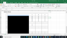
As for the second problem it should be relevant AFTER combining files, but I will share an image of how the original file looks like for Screenshot 14.. sorry I don't know how to 'embed' an excel sheet..

Under 'Institute of Mercedez' there will be a new table that references that, but the name will be different example Io Mercedez... I blacked out column D for privacy reasons but basically there are names there, and the new table should look something like in screenshot 16. For screenshot 16 it is actually something I did but manually so I'm wondering how to execute faster.

 

[winds]

Bump?

 

[Misca]

Thanks for the examples. They didn't really help me understand the data any better but I might have managed to come up with a little something to get you started.

I started by creating a dummy data file with a couple of sheets of data. Then I used Power Query to create a basic query:

let
    Source = Excel.Workbook(File.Contents("C:\TMP\DummyData.xlsx"), null, true),
    #"Filtered Rows" = Table.SelectRows(Source, each [Kind] = "Sheet"),
    #"Removed Other Columns" = Table.SelectColumns(#"Filtered Rows",{"Name", "Data"}),
    #"Expanded Data1" = Table.ExpandTableColumn(#"Removed Other Columns", "Data", {"Column1", "Column2", "Column3", "Column4", "Column5", "Column6"}, {"Column1", "Column2", "Column3", "Column4", "Column5", "Column6"}),
    #"Filled Down" = Table.FillDown(#"Expanded Data1",{"Column1"}),
    #"Renamed Columns" = Table.RenameColumns(#"Filled Down",{{"Name", "Sheet Name"}, {"Column1", "Sheet Title"}, {"Column2", "Number Column"}, {"Column3", "Name Column"}, {"Column4", "9"}, {"Column5", "10"}, {"Column6", "11"}}),
    #"Filtered Rows1" = Table.SelectRows(#"Renamed Columns", each ([Name Column] <> null))
in
    #"Filtered Rows1"

The query simply gets all the data from all the worksheets in the file and fills down the Sheet Title from Column B
I duplicated the query I made and turned it into a simple function that I named fnFileData:

(MyFileName as text)=>
let
    Source = Excel.Workbook(File.Contents(MyFileName), null, true),
    #"Filtered Rows" = Table.SelectRows(Source, each [Kind] = "Sheet"),
    #"Removed Other Columns" = Table.SelectColumns(#"Filtered Rows",{"Name", "Data"}),
    #"Expanded Data1" = Table.ExpandTableColumn(#"Removed Other Columns", "Data", {"Column1", "Column2", "Column3", "Column4", "Column5", "Column6"}, {"Column1", "Column2", "Column3", "Column4", "Column5", "Column6"}),
    #"Filled Down" = Table.FillDown(#"Expanded Data1",{"Column1"}),
    #"Renamed Columns" = Table.RenameColumns(#"Filled Down",{{"Name", "Sheet Name"}, {"Column1", "Sheet Title"}, {"Column2", "Number Column"}, {"Column3", "Name Column"}, {"Column4", "9"}, {"Column5", "10"}, {"Column6", "11"}}),
    #"Filtered Rows1" = Table.SelectRows(#"Renamed Columns", each ([Name Column] <> null))
in
    #"Filtered Rows1"

If you compare the codes you can see the only difference is at the very beginning: I simply changed the hard coded file name into a parameter called MyFileName.

Now that I had my function ready I can use it the folder query:

let
    Source = Folder.Files("C:\TMP"),
    #"Added Custom" = Table.AddColumn(Source, "Data", each fnFileData([Folder Path] & [Name])),
    #"Removed Other Columns" = Table.SelectColumns(#"Added Custom",{"Data"}),
    #"Expanded Data" = Table.ExpandTableColumn(#"Removed Other Columns", "Data", {"Sheet Name", "Sheet Title", "Number Column", "Name Column", "9", "10", "11"}, {"Sheet Name", "Sheet Title", "Number Column", "Name Column", "9", "10", "11"}),
    #"Unpivoted Other Columns" = Table.UnpivotOtherColumns(#"Expanded Data", {"Sheet Name", "Sheet Title", "Number Column", "Name Column"}, "Column Header", "Value")
in
    #"Unpivoted Other Columns"

The folder query appends all the data from all the worksheets and unpivots the columns "9", "10" and "11". I don't know if those are fixed names or what but I handlend them as if they were fixed. I don't even promote the headers but simply rename them just to skip a couple of rows.

The whole example query expects all the sheets in your workbooks to have the same data structure: If your data has different number of columns of data on each sheet you might want to use a more dynamic approach. That can be done with Power Query as well but that's a lot more work.

The folder query is not finished. You might want to pivot the data using the "Sheet Title" column to create the new columns. I didn't do it because I didn't know the meaning of the rest of the columns: The end result will be a lot cleaner if you get rid of all the extra columns before pivoting.