Highlighting Cells IF Conditions Met

[rprieto7]

Hello,

I work for a public school. We are trying to upgrade our attendance call log spreadsheet, and I was tasked w/ doing it as the tech-savvy guy. I built out the entire sheet by myself, but I have hit a snag in finishing this project.

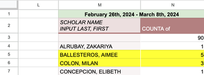
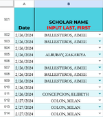
I created a bunch of pivot tables (every two weeks of school). If a student misses 3 or more days in 2 weeks, then their name gets highlighted on the pivot table. If their name gets highlighted in that specific pivot table, then I would like for that name to be flagged on the main table.

How do I highlight a cell if it matches another name in that same sheet AND if that name has previously been highlighted in the pivot table?

Thank You!

 

[awoohaw]

You'll need to probably tweak this as the PIVOT TABLE guts won't copy over with the xl2bb mini sheet.
But, essentially use the GETPIVOTDATA() Function in a Conditional Formatting Statement:
(column C is just me confirming how the CF formula will work, it is not needed in your final worksheet).

The conditional formatting formula for cell A2 is:

=GETPIVOTDATA("[Measures].[Count of Date Missed]",$E$2,"[Range].[Student]","[Range].[Student].&["&A2&"]")>=3

If you are not using the Data Model for the pivot table, then the CF formula is this:

=GETPIVOTDATA("Date Missed",$E$2,"Student",A2)>=3

Book1
	A	B	C	D	E	F	G
1	Student	Date Missed
2	YLQ	2024-02-03	FALSE		Row Labels	Count of Date Missed
3	AOA	2024-02-12	FALSE		AOA	1
4	WJK	2024-02-11	FALSE		BMF	2
5	NKG	2024-02-12	FALSE		FID	2
6	BMF	2024-02-10	FALSE		GIV	3
7	RMZ	2024-02-12	FALSE		JOU	2
8	FID	2024-02-09	FALSE		NKG	1
9	GIV	2024-02-11	TRUE		RGN	3
10	RGN	2024-02-17	TRUE		RMZ	2
11	JOU	2024-02-13	FALSE		WJK	1
12	BMF	2024-02-05	FALSE		YLQ	1
13	RMZ	2024-02-16	FALSE		Grand Total	18
14	FID	2024-02-07	FALSE
15	GIV	2024-02-07	TRUE
16	RGN	2024-02-08	TRUE
17	JOU	2024-02-11	FALSE
18	GIV	2024-02-16	TRUE
19	RGN	2024-02-08	TRUE
20	JOU	2024-02-14	FALSE
21
Sheet2

Cell Formulas
Range	Formula
C2:C20	C2	=GETPIVOTDATA("[Measures].[Count of Date Missed]",$E$2,"[Range].[Student]","[Range].[Student].&["&A2&"]")>=3

Cells with Conditional Formatting
Cell	Condition		Cell Format	Stop If True
A2:A20	Expression	=GETPIVOTDATA("[Measures].[Count of Date Missed]",$E$2," #VALUE!

#VALUE!

#VALUE!

 

[rprieto7]

That was really helpful. I am on the verge of figuring this out, but now a new problem has arised.

My pivot tables take into account "blanks" so considering there are greater than 3 blanks, it is highlighting the entire excel sheet. Is there anyway to make this formula w/ except highlighting of blanks in the conditional formatting?

 

[awoohaw]

That is a little beyond me. If you use the Data Model Pivot Table, it seems to ignore those.
If you use do not use the Data Model, go to Pivot Table Options and change the For Blank Cells Value to NA() or something like that.
(not sure it will count for you or not).

But from a data standpoint, why do you have essentially empty rows for this, unless you have other columns not related to Absences?

You may be able to filter the blank values out. But that could be time consuming.

 

[awoohaw]

There is a check box in Field Value Setting for "Show Items with No Data", but when I uncheck it, it still shows that Student Name. So strange.
I can't figure it out.

 

[rprieto7]

Howdy,

Yeah, there are a bunch of other columns not related to the absence that I am not allowed to show. That would explain it .

I was able to figure it out though while discussing this with you, so all good!

Thank You,

 

[awoohaw]

okay, happy you figured it out. Would you mind sharing your solution and marking it? If anyone searches for Conditional Formatting based on Pivot Tables they can come find it.

 

[rprieto7]

I was able to go to the pivot table and filter out the blanks. This meant that it would not be picked up by the conditional formatting, which is exactly what we wanted. I will mark this thread as resolved.

 

[awoohaw]

Great, happpy to help! Best Wishes!