Highlighting rows in a column when number changes (numbers are in consecutive order)

[mstaralynn]

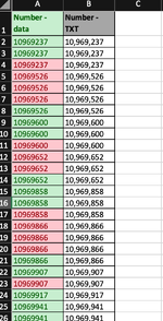
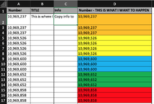
Hello - I have been trying to find a solution to this and have so far can up empty - but it seems like there HAS to be a way. I have a column with numbers in consecutive order - there could be 5 of one number, 3 of the next, 7 of the one after that - so I need to copy/paste info that correlates with the number. Problem is sometimes the numbers are similar and I miss the change and copy the wrong info. If I could have the rows colored, and change each Tim the number changes - I could visually see how far down I need to copy the info. The colors do not matter - its really just a visual guide. I tried the Conditional Formatting, Color Scales - and that doesn't work because they are in consecutive order. Also - find duplicates doesn't work either. Please see in the pic how I want the row to look - it could be the same 2 colors alternating at each number change - color doesn't matter. This is something I do very often and any way to make it easier is nice. THANK YOU!!!

 

[rollis13]

If you don't mind a macro this could be a solution. The macro tests numbers in column D and changes background color (light colors) at every change of numbers:

Option Explicit
Sub Color_Cells()
    Dim rw As Long
    Dim rndColor As Integer
    For rw = 2 To Range("D" & Rows.Count).End(xlUp).Row
        If (Cells(rw, "D") <> Cells(rw - 1, "D")) Then rndColor = Application.RandBetween(33, 45)
        With Cells(rw, "D").Interior
            .ColorIndex = rndColor
        End With
    Next rw
End Sub

 

[Trebor76]

Hi mstaralynn,

Welcome to MrExcel!!

Here's my attempt that uses light green and yellow to highlight each block in Col. A (run while on the sheet with the numbers):

Option Explicit
Sub Macro1()

    Dim objCell As Object
    Dim i As Long, j As Long
    Dim strRGB As String
   
    strRGB = "200,255,200" 'First fill colour (light green)
    j = Cells(Rows.Count, "A").End(xlUp).Row
   
    Application.ScreenUpdating = False
   
    For i = 2 To j
        Set objCell = Range("A" & i)
        If i = 2 Then 'First record
            objCell.Interior.Color = RGB(Split(strRGB, ",")(0), Split(strRGB, ",")(1), Split(strRGB, ",")(2))
        Else
            If Range("A" & i) <> Range("A" & i - 1) Then
                strRGB = IIf(strRGB = "200,255,200", "255,255,155", "200,255,200") 'Switch between light green and light yellow
            End If
            objCell.Interior.Color = RGB(Split(strRGB, ",")(0), Split(strRGB, ",")(1), Split(strRGB, ",")(2))
        End If
    Next i
   
    Application.ScreenUpdating = True

End Sub

Note though that code could actually copy the data for you so there's probably no need to do this.

Regards,

Robert

 

[mstaralynn]

Thank you! I have never ran a macro before - but will give it a shot!

 

[Peter_SSs]

Conditional formatting like this?

23 01 26.xlsm
	D
1	Number
2	5
3	5
4	5
5	5
6	5
7	3
8	3
9	7
10	7
11	7
12	7
13	7
14	6
15	45
16	45
Bands

Cells with Conditional Formatting
Cell	Condition		Cell Format	Stop If True
D2:D16	Expression	=ISEVEN(COUNT(UNIQUE(D$2:D2)))	text	NO
D2:D16	Expression	=ISODD(COUNT(UNIQUE(D$2:D2)))	text	NO

 

[Peter_SSs]

Looking again I notice that your values are left-aligned so may not be numerical. This one should work either way.

23 01 26.xlsm
	D
1	Number
2	a5
3	a5
4	a5
5	a5
6	a5
7	b3
8	b3
9	7
10	7
11	7
12	7
13	7
14	d6
15	e45
16	e45
Bands (2)

Cells with Conditional Formatting
Cell	Condition		Cell Format	Stop If True
D2:D16	Expression	=ISEVEN(ROWS(UNIQUE(D$2:D2)))	text	NO
D2:D16	Expression	=ISODD(ROWS(UNIQUE(D$2:D2)))	text	NO

Note though that both of my suggestions assume that all the same values are grouped together in the column. It would not work if values reoccur further down the column like "a5" in this sample.

23 01 26.xlsm
	D
1	Number
2	a5
3	a5
4	a5
5	a5
6	a5
7	b3
8	b3
9	7
10	7
11	7
12	7
13	7
14	a5
15	e45
16	e45
Bands (3)

 

[mstaralynn]

Yes! This looks correct. The same values are grouped together. They are numerical, but I also usually have the same values in a different column just as text. I hope this isn’t a dumb question - but is this a formula I can use?

 

[Peter_SSs]

is this a formula I can use?

You should be able to ... but the easiest way to answer that for sure would be to try it.

 

[mstaralynn]

You should be able to ... but the easiest way to answer that for sure would be to try it.

This worked almost - I was confused & then realized it was supposed to go in the conditional formatting formula place - OK - it worked BUT - the last number of a group is staying the same as the next group. Here is a pic & I think a mini-sheet?

Numbers.xlsx
	A	B
1	Number
2	10969237
3	10969237
4	10969237
5	10969526
6	10969526
7	10969526
8	10969526
9	10969600
10	10969600
11	10969600
12	10969652
13	10969652
14	10969652
15	10969858
16	10969858
17	10969858
18	10969866
19	10969866
20	10969866
21	10969866
22	10969907
23	10969907
24	10969917
25	10969941
26	10969941
27	10969941
28	10969941
29	10969941
30	10969941
31	10969941
32	10969941
33	10969941
34	10970077
35	10970077
36	10970078
37	10970078
38	10970078
39	10970078
40	10970318
41	10970318
42	10970383
43	10970383
44	10970385
45	10970385
46	10970385
47	10970385
48	10970481
49	10970518
50	10970518
51
Sheet1

Cells with Conditional Formatting
Cell	Condition		Cell Format	Stop If True
A:A	Expression	=ISODD(ROWS(UNIQUE(A$2:A2)))	text	NO
A:A	Expression	=ISEVEN(ROWS(UNIQUE(A$2:A2)))	text	NO

 

[Peter_SSs]

A couple of issues

1. You have applied Conditional Formatting to an entire column. How much data do you actually have? Since Conditional Formats are volatile I would not recommend applying them to an entire column as every time Excel recalculates for any reason the CF will have to evaluate all 2 x 1,048,576 CF formulas to determine if the cell should be formatted a particular way.
   
   
2. If you are going to apply the CF to cells below where the data is then a slight adjustment to the formula might be in order anyway.

So, in my dummy example below I have data in rows 2:12 but I want to allow for possible data down to row 20. I select from D2 (not D1) down to D20 and apply the shown CF formulas.
Is that something that you could adapt to suit your circumstances?

23 01 26.xlsm
	D
1	Number
2	a5
3	a5
4	a5
5	b3
6	b3
7	7
8	7
9	7
10	d6
11	e45
12	e45
13
14
15
16
17
18
19
20
Bands (2)

Cells with Conditional Formatting
Cell	Condition		Cell Format	Stop If True
D2:D20	Expression	=AND(ISEVEN(ROWS(UNIQUE(D$2:D2))),D2<>"")	text	NO
D2:D20	Expression	=AND(ISODD(ROWS(UNIQUE(D$2:D2))),D2<>"")	text	NO