How to find a value based on 2 criteria: one horizontal and one vertical BUT which is not always in the same column.

[smetu]

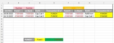
Is there a way to find a formula in the green box based on the grey and yellow boxes.
The fact that the transaction ID's of Fund I and Fund II are not in the same columns prevents me to find a solution to this problem.....
It's been a head scratching for me for weeeeks!

 

[ExceLoki]

ok... so try this:

=OFFSET(A3,(MATCH(TRUE,MMULT(IFERROR(FIND(C14,FILTER(A3:Q6,A3:Q3="transaction id n*")),0),{1;1;1;1})>0,0))-1,0)

you will need to add another "1;" to {1;1;1;1} for each time 'transaction id n*' is found in row 3

i'll post the mini sheet in a moment

 

[ExceLoki]

find a value based on 2 criteria.xlsx
	A	B	C	D	E	F	G	H	I	J	K	L	M	N	O	P	Q
1
2		sunrise	sunrise			consent	consent
3	dates	fund i	vs bank	refill	transaction id n*	fund ii	vs bank	refill	transaction id n*	fund iii	vs bank	refill	transaction id n*	fund iv	vs bank	refill	transaction id n*
4	9/28/2022	1500000	1500020	cap call 1	fundi1	1600000	1600020	refill from	fundii1	1600000	1600020	refill from	fundiii1	1600000	1600020	refill from	fundiv1
5	10/4/2022	-2500000	-2500020	cap call 2	fundi2	-3500000	-3500020	cap call 1	fundii2	-3500000	-3500020	cap call 1	fundiii2	-3500000	-3500020	cap call 1	fundiv2
6	3/23/2023				123				987				410				985
7
8
9
10
11
12
13
14			fundiii2	dates	10/4/2022	v2
15					10/4/2022	v3
final

Cell Formulas
Range	Formula
E14	E14	=INDIRECT(ADDRESS(IFERROR(IF(MATCH(C14,4:4,0),4),5),1))
E15	E15	=OFFSET(A3,(MATCH(TRUE,MMULT(IFERROR(FIND(C14,FILTER(A3:Q6,A3:Q3="transaction id n*")),0),{1;1;1;1})>0,0))-1,0)

 

[ExceLoki]

find a value based on 2 criteria.xlsx
	A	B	C	D	E	F	G	H	I	J	K	L	M	N	O	P	Q
1
2		sunrise	sunrise			consent	consent
3	dates	fund i	vs bank	refill	transaction id n*	fund ii	vs bank	refill	transaction id n*	fund iii	vs bank	refill	transaction id n*	fund iv	vs bank	refill	transaction id n*
4	9/28/2022	1500000	1500020	cap call 1	fundi1	1600000	1600020	refill from	fundii1	1600000	1600020	refill from	fundiii1	1600000	1600020	refill from	fundiv1
5	10/4/2022	-2500000	-2500020	cap call 2	fundi2	-3500000	-3500020	cap call 1	fundii2	-3500000	-3500020	cap call 1	fundiii2	-3500000	-3500020	cap call 1	fundiv2
6	3/23/2023				123				987				410				985
7
8
9
10
11
12
13
14			fundiii2	dates	10/4/2022	v2
15					10/4/2022	v3
final

Cell Formulas
Range	Formula
E14	E14	=INDIRECT(ADDRESS(IFERROR(IF(MATCH(C14,4:4,0),4),5),1))
E15	E15	=OFFSET(A3,(MATCH(TRUE,MMULT(IFERROR(FIND(C14,FILTER(A3:Q6,A3:Q3="transaction id n*")),0),{1;1;1;1})>0,0))-1,0)

btw, ignore the part in green, it's the part in yellow

 

[smetu]

Thank you very much, we are almost there!
The only thing is that instead of selecting A3, can you select D14? Because the col of the dates may change with time so the dates won't always be in col A.
I do hope you find a way!

 

[ExceLoki]

the formula is not using the cell value "dates" in d14 for anything.
the a3 in the formula is tell it where to move from to get the final value. i've edited this to now look for the value "dates" in row 3.
will your data always be starting in row 3 as in your example? if not then you'd need to make some adjustments to the formula
if it will be then you should be able to use this.
i also threw in a way to find the amount based on the fund searching for

find a value based on 2 criteria.xlsx
	A	B	C	D	E	F	G	H	I	J	K	L	M	N	O	P	Q
1
2		sunrise	sunrise			consent	consent
3	dates	fund i	vs bank	refill	transaction id n*	fund ii	vs bank	refill	transaction id n*	fund iii	vs bank	refill	transaction id n*	fund iv	vs bank	refill	transaction id n*
4	9/28/2022	1,500,000	1,500,020	cap call 1	fundi1	1,600,000	1,600,020	refill from	fundii1	1,600,000	1,600,020	refill from	fundiii1	1,600,000	1,600,020	refill from	fundiv1
5	10/4/2022	-2,500,000	-2,500,020	cap call 2	fundi2	-3,500,000	-3,500,020	cap call 1	fundii2	-3,500,000	-3,500,020	cap call 1	fundiii2	-3,500,000	-3,500,020	cap call 1	fundiv2
6	3/23/2023	test0			fundi3	test1			fundii3	test2			fundiii3	test3			985
7
8
9
10
11
12
13
14			fundii2	date	10/4/2022
15				amount	-3,500,000.00
final

Cell Formulas
Range	Formula
E14	E14	=OFFSET(INDIRECT(ADDRESS(3,MATCH("dates",3:3,0))),(MATCH(TRUE,MMULT(IFERROR(FIND(C14,FILTER(A3:Q6,A3:Q3="transaction id n*")),0),{1;1;1;1})>0,0))-1,0)
E15	E15	=OFFSET(INDIRECT(ADDRESS(3,MATCH((CONCAT(LEFT(C14,4)," ",MID(C14,5,LEN(C14)-5))),3:3,0))),(MATCH(TRUE,MMULT(IFERROR(FIND(C14,FILTER(A3:Q6,A3:Q3="transaction id n*")),0),{1;1;1;1})>0,0))-1,0)

 

[smetu]

I need please that the formula includes D14 ("Dates"), so it will return the corresponding date of the transaction ID, in a way that if I modify and write "refill" in D14, it will return then "cap call 1" automatically.
And then my goal will be achieved! Is it possible to do that, you think? Please say yes.

 

[smetu]

PS: I have counted and I have 52 funds, so 52 columns of transaction ID's as well.

 

[ExceLoki]

the values in the formula: A3:Q6 & A3:Q3 till need to be extended to fit your actual data
but the formula

=OFFSET(INDIRECT(ADDRESS(3,MATCH(D14,3:3,0))),(MATCH(TRUE,MMULT(IFERROR(FIND(C14,FILTER(A3:Q6,A3:Q3="transaction id n*")),0),{1;1;1;1;1;1;1;1;1;1;1;1;1;1;1;1;1;1;1;1;1;1;1;1;1;1;1;1;1;1;1;1;1;1;1;1;1;1;1;1;1;1;1;1;1;1;1;1;1;1;1;1})>0,0))-1,0)

should give you the results you are looking for

 

[smetu]

Thank youuuuu! You're a genious!

 

[smetu]

Last question: Is it possible to find a way without entering the 52 "1"?
Because I will add some new funds along the months.