How to rank multiple datasets by suppliers across 6 columns

[Aerobus]

Hello,

I've extensively studied the =rank page and I am still struggling,

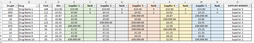
I have Product names in columns B a unique identifier in A, this is used for Vlookups of prices from 6 different suppliers and a pre determined "winner" of a price cascade.

What I need to be able to do is then, for each unique ID line (Row) rank each supplier by price there after.

So in my example attached, Rank 1 is determined by the column Supplier Winner (O).
So in the Rank column attached to Supplier 1 I need to work out what rank it places Supplier 1 as within the data that is all the supplier prices for that row.
In my example I've attached, the Rank is in the order I am trying to get it to work out,
I have 900+ lines of data so I need this to work as automatically as possible.

Then rinse and repeat for the other 5 rank columns attached to each supplier.

Right now I've been working out just which is 1st place, and the rest are 2nd - 5th, what I need to do is have what is 1st, 2nd, 3rd, 4th, 5th by supplier. Where suppliers are equal price we have a predetermined cascade that would be implemented based on the order of the formula ideally. It doesn't necessarily have to work with ranks, but as long as I can get something that works to output what I need, I don't care how convoluted it is!

Kind Regards,

 

[KRice]

Do you have any flexibility regarding the table structure? When a set of values (like the Supplier prices) are in non-contiguous columns, referring to them with functions that work well with contiguous ranges becomes problematic. You could create an array that covers cols E:N and use values only from column indexes {1,3,5,7,9} to isolate the prices into an array, but I had no luck doing much with it after that. If you restructured the table as shown, a single formula copied throughout the Ranking side of the table will return results close to what you want...but the issue remains with something you only briefly touched upon: resolution of ties. The RANK function will assign ties the same place value (see 1st line of data). What rule do you apply to resolve ties to something other than a same-number ranking?

MrExcel_20220601.xlsx
	E	F	G	H	I	J	K	L	M	N
1	Supplier 1	Supplier 2	Supplier 3	Supplier 4	Supplier 5	Rank S1	Rank S2	Rank S3	Rank S4	Rank S5
2	25.69	24.65	23.4	22.9	22.9	5	4	3	1	1
3	1.11	3.33	4.44	2.22	5.55	1	3	4	2	5
4	25.69	22.9	22.9	23.4	24.65	5	1	1	3	4
5	1.11	5.55	2.22	4.44	3.33	1	5	2	4	3
Sheet3

Cell Formulas
Range	Formula
J2:N5	J2	=RANK(E2,$E2:$I2,1)

 

[Aerobus]

Do you have any flexibility regarding the table structure? When a set of values (like the Supplier prices) are in non-contiguous columns, referring to them with functions that work well with contiguous ranges becomes problematic. You could create an array that covers cols E:N and use values only from column indexes {1,3,5,7,9} to isolate the prices into an array, but I had no luck doing much with it after that. If you restructured the table as shown, a single formula copied throughout the Ranking side of the table will return results close to what you want...but the issue remains with something you only briefly touched upon: resolution of ties. The RANK function will assign ties the same place value (see 1st line of data). What rule do you apply to resolve ties to something other than a same-number ranking?

MrExcel_20220601.xlsx
	E	F	G	H	I	J	K	L	M	N
1	Supplier 1	Supplier 2	Supplier 3	Supplier 4	Supplier 5	Rank S1	Rank S2	Rank S3	Rank S4	Rank S5
2	25.69	24.65	23.4	22.9	22.9	5	4	3	1	1
3	1.11	3.33	4.44	2.22	5.55	1	3	4	2	5
4	25.69	22.9	22.9	23.4	24.65	5	1	1	3	4
5	1.11	5.55	2.22	4.44	3.33	1	5	2	4	3
Sheet3

Cell Formulas
Range	Formula
J2:N5	J2	=RANK(E2,$E2:$I2,1)

Full flexibility on the column placement, I started to write IF formats last night but ran out of willpower to think of the logic required to work it out.

What I was trying to write is something (in each of the rank columns),
So in Supplier 1 column it would read something like
IF column O = "Supplier 1" then output "1st", If not then Rank

The actual end game is to have the first choice supplier output 0.01p, then second 0.02p, third 0.03p etc.
What can't happen is first choice having same rank as another supplier with the same price.

I will give it a go and see how it goes with more coffee and sleep.