I need to multiply the result not sum ie SUMIFS

[jmillf]

Hi please see attached screenshot.

I need to multiply the results instead of summing the results. I currently get the correct variables summing, just need a hand to multiply.

=SUMIFS(Y73:Y850,C73:C850,AF74,F73:F850,"DS")

Help pls

Thanks
Jarrad

 

[jmillf]

Sorry screenshot was terrible please see attached.

 

[sandy666]

maybe use this

 

[Peter_SSs]

I need to multiply the results instead of summing the results. I currently get the correct variables summing, just need a hand to multiply.

=SUMIFS(Y73:Y850,C73:C850,AF74,F73:F850,"DS")

Try this. It is an array formula so should be entered without the {} but confirmed with Ctrl+Shift+Enter, not just Enter. If confirmed correctly, Excel will insert the {}.

{=PRODUCT(IF(C73:C850=AF74,IF(F73:F850="DS",Y73:Y850)))}

 

[jmillf]

Thanks Peter, that did work but I have now changed what I am after ha.....

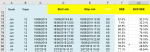
Essentially what I'm after is a formula that will average OEE number (column Y) per shift ie DS, AS, NS (column F) per day. I would like the average OEE number displayed in column AC. See expected result screenshot below.

My current formula is a bit of spaghetti (below) which doesn't currently return the correct result plus there is some background work of splitting the content of certain cells with the "Text to Columns" function.

<=IFERROR(SUMIFS(Y74:Y850,C74:C850,AF74,F74:F850,"DS")/(COUNTIFS(C74:C850, AF74,F74:F850,"DS")),"NA")>

If someone could provide some guidance it will be a great help.

Thanks
Jarrad

 

[Peter_SSs]

Could you give us something that we can easily read and copy to test with? Link already provided in post 3, or see my signature block below.

 

[jmillf]

Thanks Peter, can you let me know if the below worked.
��

 

[jmillf]

hmmmm doesn't look like it worked.

 

[Peter_SSs]

hmmmm doesn't look like it worked.

No, but I think you are close.
Take a look at this.

 

[jmillf]

Book1
	A	B	C	D	E	F																			Y				AC	AD	AE	AF
72	Month	Week		Start Job	Stop Job	Shift																			OEE				Shift OEE	Shift Performance Rate	Shift Availability
73
74	Jun	12	18/06/2019	18/06/2019 6:50:00 AM	18/06/2019 12:00:00 PM	DS																			57.3%				32.31%			18/06/2019
75	Jun	12	18/06/2019	18/06/2019 12:00:00 PM	18/06/2019 2:50:00 PM	DS																			7.4%				7.35%			18/06/2019
76	Jun	12	18/06/2019	18/06/2019 2:50:00 PM	18/06/2019 3:10:00 PM	AS																			87.5%				NA			18/06/2019
77	Jun	12	18/06/2019	18/06/2019 3:10:00 PM	18/06/2019 5:35:00 PM	AS																			68.3%				NA			18/06/2019
78	Jun	12	18/06/2019	18/06/2019 5:35:00 PM	18/06/2019 6:55:00 PM	AS																			81.3%				NA			18/06/2019
79	Jun	12	18/06/2019	18/06/2019 6:55:00 PM	18/06/2019 9:45:00 PM	AS																			61.2%				NA			18/06/2019
80	Jun	12	18/06/2019	18/06/2019 9:45:00 PM	18/06/2019 10:50:00 PM	AS																			97.6%				NA			18/06/2019
81	Jun	12	18/06/2019	18/06/2019 10:50:00 PM	19/06/2019 6:50:00 AM	NS																			84.9%				NA			18/06/2019
82	Jul	14	2/07/2019	2/07/2019 6:50:00 AM	2/07/2019 10:10:00 AM	DS																			35.4%				48.54%			2/07/2019
83	Jul	14	2/07/2019	2/07/2019 10:10:00 AM	2/07/2019 10:50:00 AM	DS																			77.1%				NA			2/07/2019
84	Jul	14	2/07/2019	2/07/2019 10:50:00 AM	2/07/2019 2:50:00 PM	DS																			33.1%				33.13%			2/07/2019
85	Jul	14	2/07/2019	2/07/2019 2:50:00 PM	2/07/2019 6:10:00 PM	AS																			33.7%				55.10%			2/07/2019
Lam 4

Cell Formulas
Range	Formula
Y74:Y85	Y74	=W74*X74
AC74:AC82, AC84	AC74	{=IFERROR(SUMIFS(Y74:Y850,C74:C850,AF74,F74:F850,"DS")/(COUNTIFS(C74:C850, AF74,F74:F850,"DS")),"NA")}
AC83	AC83	{=IFERROR(SUMIFS(Y82:Y859,C82:C859,AF83,F82:V859,"DS")/(COUNTIFS(C82:C859, AF83,F82:F859,"DS")),"NA")}
AC85	AC85	=IFERROR(SUMIFS(Y83:Y859,C83:C859,AF85,F83:F859,"DS")/(COUNTIFS(C83:C859, AF85,F83:F859,"DS")),"NA")
AF74:AF85	AF74	=C74
Press CTRL+SHIFT+ENTER to enter array formulas surrounded with curly braces.

Named Ranges
Name	Refers To	Cells
'Lam 4'!Print_Titles	='Lam 4'!$A:$H,'Lam 4'!$72:$72	AC74:AC85, AF74:AF85

Cells with Data Validation
Cell	Allow	Criteria
F73:F85	List	=$AJ$19:$AJ$21