IF(Count not working for 2 values

[The Power Loon]

I have data in columns M through Z. Based on how many columns have data in a specific row, i want column B to give it a category.

When trying to past the below formula into B2, I get window stating "there is a problem with this formula".

=IF(COUNT(M2:Z2)=1,"1st to 2nd",IF(COUNT(M2:Z2)=2,"1st to 3rd",IF(COUNT(M2:Z2)=3,"1st to 4th",IF(COUNT(M2:Z2)=4,"2nd to 3rd",IF(COUNT(M2:Z2)=5,"2nd to 4th”,IF(COUNT(M2:Z2)=6,"3rd to 4th”,IF(COUNT(M2:Z2)=7,"1st to 2nd E3",IF(COUNT(M2:Z2)=8,"1st to 2nd E4",IF(COUNT(M2:Z2)=9,"1st to 3rd E4",IF(COUNT(M2:Z2)=10,"2nd to 3rd E4",IF(COUNT(M2:Z2)=11,"Open, E2",IF(COUNT(M2:Z2)=12,"Open, E3",IF(COUNT(M2:Z2)=13,"Open, E4",IF(COUNT(M2:Z2)=14,"Open, EEOD",""))))))))))))))

However, when i remove the "IF(Count" for 5 and 6 (bolded above) and the respective closing parenthesis, it works.

I've tried changing the resulting value, retyping it out, and placing it elsewhere in the formula without success. Any thoughts on why this doesn't work, and/or a solution?

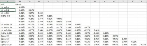
Picture contains a sample of issue

 

[Fluff]

You have the wrong type of quotes after the text in both the bold sections

 

[hrayani]

=IF(COUNT(M2:Z2)=1,"1st to 2nd",IF(COUNT(M2:Z2)=2,"1st to 3rd",IF(COUNT(M2:Z2)=3,"1st to 4th",IF(COUNT(M2:Z2)=4,"2nd to 3rd",IF(COUNT(M2:Z2)=5,"2nd to 4th",IF(COUNT(M2:Z2)=6,"3rd to 4th",IF(COUNT(M2:Z2)=7,"1st to 2nd E3",IF(COUNT(M2:Z2)=8,"1st to 2nd E4",IF(COUNT(M2:Z2)=9,"1st to 3rd E4",IF(COUNT(M2:Z2)=10,"2nd to 3rd E4",IF(COUNT(M2:Z2)=11,"Open, E2",IF(COUNT(M2:Z2)=12,"Open, E3",IF(COUNT(M2:Z2)=13,"Open, E4",IF(COUNT(M2:Z2)=14,"Open, EEOD",""))))))))))))))

 

[Fluff]

You could simplify the formula using Choose

=CHOOSE(IF(COUNT(M2:Z2)=0,15,COUNT(M2:Z2)),"1st to 2nd","1st to 3rd","1st to 4th","2nd to 3rd","2nd to 4th","3rd to 4th","1st to 2nd E3","1st to 2nd E4","1st to 3rd E4","2nd to 3rd E4","Open, E2","Open, E3","Open, E4","Open, EEOD","")

 

[The Power Loon]

You have the wrong type of quotes after the text in both the bold sections

That's what I get for typing up my formulas outside of excel. Thank you for resolving this issue.

 

[jasonb75]

This would be much easier with a lookup table, that many nested functions is a recipe for failure.

First list out all of the possible outcomes, starting with a count of 1, lets say with 1st to 2nd in AA2, then the rest of the results in order down the column.

Then it would be as simple as

=INDEX($AA$2:$AA$15,COUNT(M2:Z2))

in B2 and filled down.

edit:- might be better with

=IF(M2="","",INDEX($AA$2:$AA$15,COUNT(M2:Z2)))

to allow for no data at all in the row.

 

[Fluff]

Glad we could help & thanks for the feedback.

 

[The Power Loon]

You could simplify the formula using Choose

=CHOOSE(IF(COUNT(M2:Z2)=0,15,COUNT(M2:Z2)),"1st to 2nd","1st to 3rd","1st to 4th","2nd to 3rd","2nd to 4th","3rd to 4th","1st to 2nd E3","1st to 2nd E4","1st to 3rd E4","2nd to 3rd E4","Open, E2","Open, E3","Open, E4","Open, EEOD","")

I didn't realize the Choose function could be used that way. I'll have to keep this in mind. Thank you for posting it