IF formula to create Eisenhower Matrix

[Grishma]

Hi everyone,

My knowledge of excel is minimal and looking to get some help here.

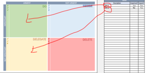
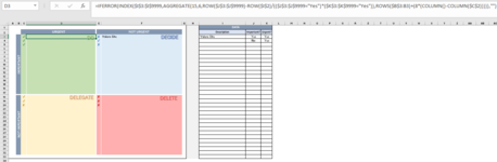
I’m creating a formula where I have the datasheet with three columns – description, important & urgent.
I want the data (description) to be populated automatically when I select yes/no from the important/urgent column.

I have attached an image that I was looking to do!

I'd greatly appreciate your help here.

 

[Toadstool]

Hi Grishma,

This does a 3x8 grid and changes will be neeed for a different sized grid... and it's not pretty.

Grishma.xlsx
	A	B	C	D	E	F	G	H	I	J	K	L
1		Urgent				Not Urgent				Description	Important	Urgent
2										Site1	Yes	No
3	Important	Site3				Site1				Site2	No	Yes
4						Site6				Site3	Yes	Yes
5						Site7				Site4	No	No
6						Site8				Site5	No	Yes
7						Site9				Site6	Yes	No
8						Site10				Site7	Yes	No
9										Site8	Yes	No
10										Site9	Yes	No
11										Site10	Yes	No
12	Not Important	Site2				Site4
13		Site5
14
15
16
17
18
19
20
Sheet1

Cell Formulas
Range	Formula
B3:D10	B3	=IFERROR(INDEX($J$2:$J$9999,AGGREGATE(15,6,ROW($J$2:$J$9999)-ROW($J$1)/(($K$2:$K$9999="Yes")*($L$2:$L$9999="Yes")),ROWS($A$3:A3)+(8*(COLUMN()-COLUMN($B$1))))),"")
F3:H10	F3	=IFERROR(INDEX($J$2:$J$9999,AGGREGATE(15,6,ROW($J$2:$J$9999)-ROW($J$1)/(($K$2:$K$9999="Yes")*($L$2:$L$9999="No")),ROWS($A$3:E3)+(8*(COLUMN()-COLUMN($F$1))))),"")
J2:J11	J2	="Site"&ROW()-1
B12:D19	B12	=IFERROR(INDEX($J$2:$J$9999,AGGREGATE(15,6,ROW($J$2:$J$9999)-ROW($J$1)/(($K$2:$K$9999="No")*($L$2:$L$9999="Yes")),ROWS($A$12:A12)+(8*(COLUMN()-COLUMN($B$1))))),"")
F12:H19	F12	=IFERROR(INDEX($J$2:$J$9999,AGGREGATE(15,6,ROW($J$2:$J$9999)-ROW($J$1)/(($K$2:$K$9999="No")*($L$2:$L$9999="No")),ROWS($A$12:E12)+(8*(COLUMN()-COLUMN($F$1))))),"")

 

[Grishma]

Wow, that's something! Thank you so much for taking the time out to look at this for me.

Somehow, it's not working for me. It kept giving me blank rows and it doesn't update on its own!

 

[Toadstool]

You can see my first entry "Site3" is in cell B3. What would be the first cell on your sheet?

How big is each quadrant? i.e. how many cells wide and down?

Which column should contain "Description"? (I'm using J.

Give me those answers and I'll build one to match your data.

 

[Grishma]

I appreciate your efforts here. I have attached an image to answer your questions!
Thanks,
G

 

[Fluff]

How about

+Fluff 1.xlsm
	A	B	C	D	E	F	G	H	I	J	K
1			Urgent		Not Urgent
2									Description	Important	Urgent
3		Important		Site4		Site2			Site2	Yes	No
4						Site7			Site3	No	Yes
5						Site8			Site4	Yes	Yes
6						Site9			Site5	No	No
7						Site10			Site6	No	Yes
8						Site11			Site7	Yes	No
9									Site8	Yes	No
10									Site9	Yes	No
11									Site10	Yes	No
12		Not Important		Site3		Site5			Site11	Yes	No
13				Site6
14
15
16
17
18
19
20
Lists

Cell Formulas
Range	Formula
D3:D10	D3	=IFERROR(INDEX($I$3:$I$1000,AGGREGATE(15,6,(ROW($I$3:$I$1000)-ROW($I$3)+1)/($J$3:$J$1000="Yes")/($K$3:$K$1000="Yes"),ROWS(D$3:D3))),"")
F3:F10	F3	=IFERROR(INDEX($I$3:$I$1000,AGGREGATE(15,6,(ROW($I$3:$I$1000)-ROW($I$3)+1)/($J$3:$J$1000="Yes")/($K$3:$K$1000="No"),ROWS(D$3:D3))),"")
I3:I12	I3	="Site"&ROW()-1
D12:D19	D12	=IFERROR(INDEX($I$3:$I$1000,AGGREGATE(15,6,(ROW($I$3:$I$1000)-ROW($I$3)+1)/($J$3:$J$1000="No")/($K$3:$K$1000="Yes"),ROWS(D$3:D3))),"")
F12:F19	F12	=IFERROR(INDEX($I$3:$I$1000,AGGREGATE(15,6,(ROW($I$3:$I$1000)-ROW($I$3)+1)/($J$3:$J$1000="No")/($K$3:$K$1000="No"),ROWS(D$3:D3))),"")

 

[Toadstool]

Unfortunately I don't have TEXTJOIN in my Excel 2016 so cannot build the responses into a single cell.

This example has 7x15 so space for 105 responses in each quadrant.

Grishma2.xlsx
	A	B	C	D	E	F	G	H	I	J	K	L	M	N	O	P	Q	R	S	T	U
1																			Description	Important	Urgent
2			Urgent								Not Urgent								Site1	Yes	No
3		Important	Site21	Site82	Site97						Site1	Site16							Site2	Yes	No
4			Site68	Site83	Site98						Site2	Site17							Site3	Yes	No
5			Site69	Site84	Site99						Site3	Site18							Site4	Yes	No
6			Site70	Site85	Site100						Site4	Site19							Site5	Yes	No
7			Site71	Site86	Site101						Site5	Site20							Site6	Yes	No
8			Site72	Site87	Site102						Site6								Site7	Yes	No
9			Site73	Site88	Site103						Site7								Site8	Yes	No
10			Site74	Site89	Site104						Site8								Site9	Yes	No
11			Site75	Site90	Site105						Site9								Site10	Yes	No
12			Site76	Site91	Site106						Site10								Site11	Yes	No
13			Site77	Site92	Site107						Site11								Site12	Yes	No
14			Site78	Site93							Site12								Site13	Yes	No
15			Site79	Site94							Site13								Site14	Yes	No
16			Site80	Site95							Site14								Site15	Yes	No
17			Site81	Site96							Site15								Site16	Yes	No
18																			Site17	Yes	No
19		Not Important	Site22	Site37							Site42	Site57							Site18	Yes	No
20			Site23	Site38							Site43	Site58							Site19	Yes	No
21			Site24	Site39							Site44	Site59							Site20	Yes	No
22			Site25	Site40							Site45	Site60							Site21	Yes	Yes
23			Site26	Site41							Site46	Site61							Site22	No	Yes
24			Site27								Site47	Site62							Site23	No	Yes
25			Site28								Site48	Site63							Site24	No	Yes
26			Site29								Site49	Site64							Site25	No	Yes
27			Site30								Site50	Site65							Site26	No	Yes
28			Site31								Site51	Site66							Site27	No	Yes
29			Site32								Site52	Site67							Site28	No	Yes
30			Site33								Site53								Site29	No	Yes
31			Site34								Site54								Site30	No	Yes
32			Site35								Site55								Site31	No	Yes
33			Site36								Site56								Site32	No	Yes
Sheet1

Cell Formulas
Range	Formula
C3:I17	C3	=IFERROR(INDEX($S$2:$S$10013,AGGREGATE(15,6,ROW($S$2:$S$10013)-ROW($S$1)/(($T$2:$T$10013="Yes")*($U$2:$U$10013="Yes")),ROWS($B$3:B3)+(15*(COLUMN()-COLUMN($C$2))))),"")
K3:Q17	K3	=IFERROR(INDEX($S$2:$S$10013,AGGREGATE(15,6,ROW($S$2:$S$10013)-ROW($S$1)/(($T$2:$T$10013="Yes")*($U$2:$U$10013="No")),ROWS($B$3:J3)+(15*(COLUMN()-COLUMN($K$2))))),"")
C19:I33	C19	=IFERROR(INDEX($S$2:$S$10013,AGGREGATE(15,6,ROW($S$2:$S$10013)-ROW($S$1)/(($T$2:$T$10013="No")*($U$2:$U$10013="Yes")),ROWS($B$19:B19)+(15*(COLUMN()-COLUMN($C$2))))),"")
K19:Q33	K19	=IFERROR(INDEX($S$2:$S$10013,AGGREGATE(15,6,ROW($S$2:$S$10013)-ROW($S$1)/(($T$2:$T$10013="No")*($U$2:$U$10013="No")),ROWS($B$19:J19)+(15*(COLUMN()-COLUMN($K$2))))),"")
S2:S33	S2	="Site"&ROW()-1

 

[Grishma]

The problem is all the site name is different, and it's not always in order. Sometimes it's lot 28, or sometimes it's some random street name. That's throwing off my formula. I see that it works great on the first section, but the next ones give me a blank one.

 

[Grishma]

And the other issue is since it's not a range, it doesn't read when you change its status from Not to Yes or otherwise.

 

[Fluff]

Who are you talking to? also what do you mean by

since it's not a range