Index and Match between Two Dates

matthewlouis

Active Member
Joined
Mar 28, 2014
Messages
374
Office Version
  1. 365
  2. 2019
Platform
  1. Windows
Hey EXCEL experts, I need a formula for an index and match that looks for a number that is below another cell number. Attached is an image with more explanation. The key is to keep the index / match between the two dates on the sheet in each column.

Thanks in advance!
 

Excel Facts

Control Word Wrap
Press Alt+Enter to move to a new row in a cell. Lets you control where the words wrap.
Hi Matthew,

Firstly your image seems to have disappeared, but I think I understood the question. If I'm right you're trying to find the minimum Closing figure that occurs between two dates. IN which case this formula should help:

=MIN((A1:A81>=F6)*(A1:A81<=F7)*(B1:B81)+NOT((A1:A81>=F6)*(A1:A81<=F7))*MAX((B1:B81)+1))

you'll need to adjust the ranges to suit your data so that:
A1:A81 are the date cells,
F6 is your earliest date,
F7 is you latest date, and
B1:B81 is you closing figure.

To find the date on which the closing figure occurs do a simply match to the figure and index to the left one column.

HTH
 
Upvote 0
PS. I should have said you need to enter that formula with CTRL-SHFT-ENTER as it is an array formula. (obviously time for bed!)
 
Upvote 0
Thanks for your quick response! Hmmmmm . . . I did that with the CTRL-SHFT-ENTER and this is what I got . . . hope the image shows. The number is incorrect, it should be 3,002.10.

3,387.15 isn't even in Column F anywhere (?) Wonder how it returned it?
 

Attachments

  • 22.png
    22.png
    127.8 KB · Views: 38
Upvote 0
First point is that for whatever reason the formula hasn’t been entered as an array formula as it is missing the {} around it. The formula needs to be editable in the formula bar and then press CTRL-SHFT-ENTER. The curly brackets should then appear.

Are you able to share the sheet?
 
Upvote 0
Hi Matthew,

Now had the chance to try some more. Not sure why you getting the result you are. My table and formula lare as shown below. The key think to not is the curly brackets around the formula, which occurs when CTRL-SHFT-ENTER is used to enter the formula, your screen shot shows these are missing.

The formula to find the Date Daily Closed Under is: =OFFSET($B$15,MATCH(I$7,$F$16:$F$10000,0),0)

Not sure why you're getting 3387.15 though as without the proper array formula entry I get #VALUE error. However, the figure itself is probably the maximum +1 which is what I use to mask out all the figures outside of the date range of interest - its the bit of the formula that starts with 'NOT(...'. Interestingly, if there was no data between the dates specified then it would return the Max+1 as that would appear to be the minimum, which might be a problem, though we can sort it.

For info, I would be tempted to convert the source data to a Table, import to PowerQuery and then use PowerPivot to produce the output. But that would require quite a bit more work :).

HTH

1593859890511.png
 
Upvote 0
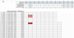
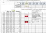
Thank you for attention to this. While I was able to fix and get the correct result of 3,002.10, when I copied and pasted the array across multiple rows, it gives me the lowest value in that column that closed under the low. I did NOT explain better what I was looking for . . . I need the FIRST number the closes UNDER that low, not the lowest number under that close. I apologize. There are a lot of moving parts to my trading system and I need to know the FIRST number that closes under that low on June 2, 2020. Yes, the correct answer for that column is 3,002.10. But it's now giving me the lowest low (MIN?) in all the other columns . . . Attached is an image with the correct numbers to the far right on a couple of other examples. But your array gives the lowest, not these numbers. So I should have said, "return the first number from column F that closes below the I2 low from that date and that first low must come from the closes between I2 and I3. Sometimes, the answer is nothing because the range (60 bars) doesn't have a close below the low from date I2. That's why you see blanks on some of those in the image. If I need to send you the spreadsheet, how do I attach?
 

Attachments

  • 742020.png
    742020.png
    99 KB · Views: 10
Last edited:
Upvote 0
In other words, if there isn't a low in that 60 day range that closed under I2, it should return a blank. Sorry, I moved the date for I3 down, it's now I9
 
Upvote 0
I have the spreadsheet ready to attach -- how do you attach it? I just see mage and URL (?)
 
Upvote 0
hmmm, actually I think you did explain what you wanted in the original post, I just didn't understand. I think what you want is a more difficult challenge - and is therefore interesting! I've seen spreadsheets attached using dropbox if that helps.

I'm not sure how I'll tackle this challenge, but I would think its possible!
 
Upvote 0

Forum statistics

Threads
1,212,934
Messages
6,110,762
Members
448,295
Latest member
Uzair Tahir Khan

We've detected that you are using an adblocker.

We have a great community of people providing Excel help here, but the hosting costs are enormous. You can help keep this site running by allowing ads on MrExcel.com.
Allow Ads at MrExcel

Which adblocker are you using?

Disable AdBlock

Follow these easy steps to disable AdBlock

1)Click on the icon in the browser’s toolbar.
2)Click on the icon in the browser’s toolbar.
2)Click on the "Pause on this site" option.
Go back

Disable AdBlock Plus

Follow these easy steps to disable AdBlock Plus

1)Click on the icon in the browser’s toolbar.
2)Click on the toggle to disable it for "mrexcel.com".
Go back

Disable uBlock Origin

Follow these easy steps to disable uBlock Origin

1)Click on the icon in the browser’s toolbar.
2)Click on the "Power" button.
3)Click on the "Refresh" button.
Go back

Disable uBlock

Follow these easy steps to disable uBlock

1)Click on the icon in the browser’s toolbar.
2)Click on the "Power" button.
3)Click on the "Refresh" button.
Go back
Back
Top