Hello,
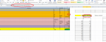
I would like to compare value in D6 with values in first column of table F10:G25 and when found just write down the value on right side in second column. I tried to use =INDEX(F10:G25,MATCH(D6,F10:F25),2) (cell F7) and then also
=INDEX(G10:G25,POZVYHLEDAT(D6,F10:F25,0),1) (which is G7), but in first case (F7) it shows correct values up to number 0.65 a writes number 275 but from value 0.7 (that should be 308) writes value above again 275, for 0.75 it writes again value one cell above 308 and value 0.8 writes one above 347 instead of 394. With function on F7 the values are correct also up to 0.65 and for 0.7 and above NOT_AVALABLE.
Can someone please help me?
Here is the sheet: Gofile - File sharing platform, anonymous and free
(Please note that it was written in czech so you might need to convert it into English version, we use ; for , and function MATCH is POZVYHLEDAT)
Thank you!
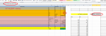