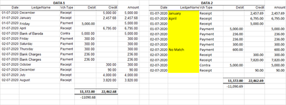
You say that the yellow cells in column J are all incorrect & I understand your reasoning. My question is why is cell I8 not
also yellow?
That row is the
second 'Bank Statement' row with 01-07-2020/Payment/5000 when there is only
one such row in the 'Own Account' section?
So ..
- If I8 is correct showing "Friday", can you give the reasoning behind that?
- If I8 should not show "Friday", what should it show?
There is a similar situation further down where there are 3 rows on the left but 4 rows the same on the right.
| RAJESH1960.xlsm |
|---|
|
|---|
| A | B | C | D | E | F | G | H | I | J | K | L | M |
|---|
| 1 | | OWN ACCOUNT | | | | | | | BANK STATEMENT | | | | |
|---|
| 2 | Date | LedgerName | Vch Type | Debit | Credit | Amount | | Date | LedgerName | Vch Type | Debit | Credit | Amount |
|---|
| 3 | 01-07-2020 | December | Receipt | | 5000 | 5000 | | 01-07-2020 | December | Receipt | | 5000 | 5000 |
|---|
| 4 | 01-07-2020 | February | Receipt | | 200 | 200 | | 01-07-2020 | February | Receipt | | 200 | 200 |
|---|
| 5 | 01-07-2020 | Friday | Payment | 5000 | | 5000 | | 01-07-2020 | Friday | Payment | 5000 | | 5000 |
|---|
| 6 | 01-07-2020 | April | Receipt | | 5000 | 5000 | | 01-07-2020 | December | Receipt | | 5000 | 5000 |
|---|
| 7 | 01-07-2020 | Bank of Baroda | Contra | 5000 | | 5000 | | 01-07-2020 | Bank of Baroda | Contra | 5000 | | 5000 |
|---|
| 8 | 01-07-2020 | Friday | Payment | 2500 | | 2500 | | 01-07-2020 | Friday | Payment | 5000 | | 5000 |
|---|
| 9 | 01-07-2020 | Saturday | Payment | 2500 | | 2500 | | 01-07-2020 | Bank of Baroda | Contra | 5000 | | 5000 |
|---|
| 10 | 01-07-2020 | Kotak Mahindra Bank | Contra | 5000 | | 5000 | | 02-07-2020 | Thursday | Payment | 5000 | | 5000 |
|---|
| 11 | 02-07-2020 | Thursday | Payment | 5000 | | 5000 | | 02-07-2020 | Thursday | Payment | 5000 | | 5000 |
|---|
| 12 | 02-07-2020 | Bank Charges | Payment | 5000 | | 5000 | | 02-07-2020 | Thursday | Payment | 5000 | | 5000 |
|---|
| 13 | 02-07-2020 | Bank Charges | Payment | 5000 | | 5000 | | 02-07-2020 | December | Receipt | | 5000 | 5000 |
|---|
| 14 | 02-07-2020 | October | Receipt | | 2500 | 2500 | | 02-07-2020 | December | Receipt | | 5000 | 5000 |
|---|
| 15 | 02-07-2020 | October | Receipt | | 2500 | 2500 | | 02-07-2020 | December | Receipt | | 5000 | 5000 |
|---|
| 16 | 02-07-2020 | December | Receipt | | 5000 | 5000 | | 02-07-2020 | December | Receipt | | 5000 | 5000 |
|---|
| 17 | 02-07-2020 | July | Receipt | | 5000 | 5000 | | | | | | | |
|---|
| 18 | 02-07-2020 | August | Receipt | | 5000 | 5000 | | | | | | | |
|---|
|
|---|
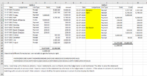
In case the yellow cells in my sheet above are incorrect too, then you could check to see if this does what you want.
| RAJESH1960.xlsm |
|---|
|
|---|
| A | B | C | D | E | F | G | H | I | J | K | L | M |
|---|
| 1 | | OWN ACCOUNT | | | | | | | BANK STATEMENT | | | | |
|---|
| 2 | Date | LedgerName | Vch Type | Debit | Credit | Amount | | Date | LedgerName | Vch Type | Debit | Credit | Amount |
|---|
| 3 | 01-07-2020 | December | Receipt | | 5000 | 5000 | | 01-07-2020 | December | Receipt | | 5000 | 5000 |
|---|
| 4 | 01-07-2020 | February | Receipt | | 200 | 200 | | 01-07-2020 | February | Receipt | | 200 | 200 |
|---|
| 5 | 01-07-2020 | Friday | Payment | 5000 | | 5000 | | 01-07-2020 | Friday | Payment | 5000 | | 5000 |
|---|
| 6 | 01-07-2020 | April | Receipt | | 5000 | 5000 | | 01-07-2020 | April | Receipt | | 5000 | 5000 |
|---|
| 7 | 01-07-2020 | Bank of Baroda | Contra | 5000 | | 5000 | | 01-07-2020 | Bank of Baroda | Contra | 5000 | | 5000 |
|---|
| 8 | 01-07-2020 | Friday | Payment | 2500 | | 2500 | | 01-07-2020 | | Payment | 5000 | | 5000 |
|---|
| 9 | 01-07-2020 | Saturday | Payment | 2500 | | 2500 | | 01-07-2020 | Kotak Mahindra Bank | Contra | 5000 | | 5000 |
|---|
| 10 | 01-07-2020 | Kotak Mahindra Bank | Contra | 5000 | | 5000 | | 02-07-2020 | Thursday | Payment | 5000 | | 5000 |
|---|
| 11 | 02-07-2020 | Thursday | Payment | 5000 | | 5000 | | 02-07-2020 | Bank Charges | Payment | 5000 | | 5000 |
|---|
| 12 | 02-07-2020 | Bank Charges | Payment | 5000 | | 5000 | | 02-07-2020 | Bank Charges | Payment | 5000 | | 5000 |
|---|
| 13 | 02-07-2020 | Bank Charges | Payment | 5000 | | 5000 | | 02-07-2020 | December | Receipt | | 5000 | 5000 |
|---|
| 14 | 02-07-2020 | October | Receipt | | 2500 | 2500 | | 02-07-2020 | July | Receipt | | 5000 | 5000 |
|---|
| 15 | 02-07-2020 | October | Receipt | | 2500 | 2500 | | 02-07-2020 | August | Receipt | | 5000 | 5000 |
|---|
| 16 | 02-07-2020 | December | Receipt | | 5000 | 5000 | | 02-07-2020 | | Receipt | | 5000 | 5000 |
|---|
| 17 | 02-07-2020 | July | Receipt | | 5000 | 5000 | | | | | | | |
|---|
| 18 | 02-07-2020 | August | Receipt | | 5000 | 5000 | | | | | | | |
|---|
|
|---|