Look Up Functions - Variable Index Numbers

[GC_EV]

Hi,

I have a workbook that contains two sheets.

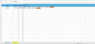
Sheet 1. PONumbers
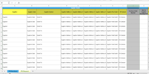
Sheet 2. PORequest

I am trying to find a way to look up a reference in Sheet 2 (Column A), find a match in Sheet 1 (Column A), then return the value of the last populated cell in the row.

I have tried Vlookup, but as the column index number will vary with each look up, it isn't sufficient for the task at hand.
I have also changed the layout of Sheet 1 and tried Hlookup, but again the variable index number is making me hit a wall.

Can you please advise if there is a way to obtain my data using a lookup function? If not, please can you advise of an alternative method to obtain the data?


Example Information
Sheet 1 contains a list of Supplier/Supplier Codes with corresponding PO Numbers.
Sheet 2 is populated automatically by either Data Validation List or Vlookup function.

In this example, I would like Sheet 2 J3, to display the data from Sheet 1 (highlighted in orange) depending on which supplier is selected in Sheet 1 Column A.
Selecting Supplier 1 would return data from Sheet 1 J2.
Selecting Supplier 2 would return data from Sheet 1 G3.
So on and so forth for future suppliers/po numbers.

Further Notes
The layout of the data in Sheet 1 can be adjusted. Sheet 2 needs to remain the same.
The data in Sheet 1 will eventually extend down Column A and across the related rows to an unknown range.

I am manually creating PO numbers in Sheet 1 by using the drag function to increase the number by 1 each time.
I then copy and paste this number into the relevant cell in Sheet 2, Column J.
This method is temporary, my next challenge is to learn how to automate this - I am not sure if this impacts my query.


Thanks

 

[GC_EV]

Images for Sheet 1 and Sheet 2.

 

[RobP]

Hi, looking at your data approach in Sheet 1, I'd say you're creating a bit of a monster.

The best way for you would be to put all your POs in column D, rather than spread them across the columns. Then of course column A & B would have duplicate data for each row (or new PO).

The reasons for doing so are two fold:

a) because then you can just use Vlookup in your columns very quickly and easily, or just filter the data you want.
b) the spreadsheet file size will be maintained at its optimum (your way, you could have 300 suppliers with 2 PO's, and 1 supplier with 250 PO's across the page. thats lots of unneccesary storage space your sheet has to deal with for a pile of potentially blank rows.

Is that something you can re-arrange your sheet into ?
cheers
Rob

 

[GC_EV]

Hi, looking at your data approach in Sheet 1, I'd say you're creating a bit of a monster.

The best way for you would be to put all your POs in column D, rather than spread them across the columns. Then of course column A & B would have duplicate data for each row (or new PO).

The reasons for doing so are two fold:

a) because then you can just use Vlookup in your columns very quickly and easily, or just filter the data you want.
b) the spreadsheet file size will be maintained at its optimum (your way, you could have 300 suppliers with 2 PO's, and 1 supplier with 250 PO's across the page. thats lots of unneccesary storage space your sheet has to deal with for a pile of potentially blank rows.

Is that something you can re-arrange your sheet into ?
cheers
Rob

Hi Rob,

Thanks for getting back to me, really appreciate the help. This site is an amazing resource for learners!

I think your approach is what I have tried previously, but then messed it up by changing to Hlookup when I should have stuck with Vlookup.

Completely agree with the monster comment, I am open to rearranging Sheet 1 to whatever is needed.

Going on what you said above, would it then be possible to do another lookup in column C, so the PO Sequence shows as the last PO number for that supplier?
I am trying to avoid duplicating the PO numbers and my temporary fix of dragging the cell across the suppliers row is going to fall apart once all PO's are in column D.

Final aim is that once the user selects the supplier in sheet 2, the next PO number for that supplier will generate in sheet 2.

 

[RobP]

Hi,

looking at the way you have written your data - looks like you are wanting to issue a unique sequence of PO number to each supplier. I would recommend a re-think on that, as in my experience, business auditors, accountants, tax authorities etc. don't like to see "broken sequences" in this kind of scenario (and invoices alike), as it implies some "not so standard practices" are being used lets say. In a previous life, when I was in a purchasing function myself, usually, you would have One single PO sequence of numbers - as it means everything can be traced and tracked forwards and backwards.

I have an example below of your layout, and I used a formula in Col C below to get the last PO (which for me is then easy, as its the one with the highest number) attached to each supplier.

Book1
	A	B	C	D
1	Supplier	Supplier Code	PO Sequence	PO Number
2	Supplier 1	EVSC_001	1004	PO001001
3	Supplier 2	EVSC_002	1002	PO001002
4	Supplier 3	EVSC_003	1005	PO001003
5	Supplier 1	EVSC_001	1004	PO001004
6	Supplier 3	EVSC_003	1005	PO001005
PO Numbers

Cell Formulas
Range	Formula
C2:C6	C2	= MAX(VALUE(SUBSTITUTE(FILTER(D:D,A:A=A2 ),"PO","")))

Essentially it generates a list (in memory) of all the PO's issued to each supplier. Then it removes the "PO" text with SUBSTITUTE(), converts the backend chars to numbers with VALUE() and looks for the highest number using MAX(). It returns this number back to Col C as your answer.

You can note, that I've only returned the numerical part of your PO - so you can quickly see that the "PO00" that you added beforehand has absolutely no use, except to make you type 4 more chars everytime you want to type it. You might want to consider dropping those, and just use simple numerical values (computers prefer plain numbers).

if you chose to do that, you could use this formula instead (basically losing the VALUE and SUBSTITUTE portions)

= MAX(FILTER(D:D,A:A=A2 ))

If you really wanted to keep "PO" in front of your numbers, then you can replace the "=" at the start of either formula with this :

="PO" &

. It basically says put PO at the start, and append the rest of the formula above to it.

Then for your sheet 2 (PO Request) - I have used this formula in cell J3

=XLOOKUP(B3,'PO Numbers'!B:B,'PO Numbers'!C:C,"Supplier Not Found")

It uses the supplier code to lookup, rather than the supplier name (as codes are usually shorter to type, and more reliable in terms of manual entry keystrokes.

Hope it answers much of your question with useful guidance.

Rob

 

[GC_EV]

Thanks Rob, sorry I am so late in responding. My deadlines were changed from end of year to this month, so have been frantically trying to develop multiple systems and procedures until the early hours.

You comment on the broken sequences was the key to unlock a lot of my issues across this and other systems. I've changed it now so all supplier numbers are sequential and am able to use power query to access a shared drive master file which contains all the PO numbers.

Due to deadline constraints I have had to limit this to manually dragging down and copy and pasting into request files received, which has eliminated the main problem of avoiding duplicates (automating was more of a convenience thing).
So, although I haven't used your above formula and explanation in this scenario, it has helped me out in other areas and saved me a lot of google time.

I just want to say thank you to yourself personally and any other members who's posts have helped over the last 4 few weeks.
I have gone from panicking when an error message pops up, to being fairly competent in VBA and excel functions, all because of the help on this site.

 

[RobP]

you're welcome .. glad to have been of assistance...

Rob