a countifs() may work
how do you know the date
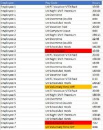
what are you using in conditional formatting
what are the possible entries for sickness - you have red and orange highlighted
something like
COUNTIFS( RANGE of employes , employee to look for , range of codes , "*"&"SICK"&"*")
or you can , include in a list of employees
| Book11 |
|---|
|
|---|
| A | B | C | D | E | F |
|---|
| 1 | | | | | | |
|---|
| 2 | | name1 | Working | | name1 | 0 |
|---|
| 3 | | name2 | Working | | name2 | 1 |
|---|
| 4 | | name3 | Working | | name3 | 0 |
|---|
| 5 | | name1 | Working | | | |
|---|
| 6 | | name2 | sick | | | |
|---|
| 7 | | name3 | Working | | | |
|---|
| 8 | | name1 | Working | | | |
|---|
| 9 | | name2 | Working | | | |
|---|
| 10 | | name3 | Working | | | |
|---|
|
|---|
OR combined with an IF()
| Book11 |
|---|
|
|---|
| A | B | C | D | E | F |
|---|
| 1 | | | | | | |
|---|
| 2 | | name1 | Working | | name1 | |
|---|
| 3 | | name2 | Working | | name2 | Off Sick |
|---|
| 4 | | name3 | Working | | name3 | |
|---|
| 5 | | name1 | Working | | | |
|---|
| 6 | | name2 | sick | | | |
|---|
| 7 | | name3 | Working | | | |
|---|
| 8 | | name1 | Working | | | |
|---|
| 9 | | name2 | Working | | | |
|---|
| 10 | | name3 | Working | | | |
|---|
|
|---|
Note: Images are difficult to see , and also requires that I input all the data myself, which means I may make an error, which is very time consuming, and from my point of view less likely to get a response, if a complicated spreadsheet. Plus we cannot see any of the formulas used.
Therefore -
A SMALL sample spreadsheet, around 10-20 rows, would help a lot here, with all sensitive data removed, and expected results mocked up and manually entered, with a few notes of explanation.
This will possibly enable a quicker and more accurate solution for you.
MrExcel has a tool called “XL2BB” that lets you post samples of your data and will allow us to copy/paste your sample data into our Excel spreadsheets, saving a lot of time.
Excel 'mini-sheet' in messages - XL2BB Although experts prefer to read your description and question instead of working in your actual file to solve your problem, there are times that it is difficult to explain an issue without providing actual...

www.mrexcel.com
You can also test to see if it works ok, in the "Test Here" forum.
Use this forum to test your signature, learn bbcode, smilies, XL2BB, etc. Threads in this forum are automatically deleted after no replies for seven (7) days
www.mrexcel.com
OR if you cannot get XL2BB to work, or have restrictions on your PC
then put the sample spreadsheet onto a share
I only tend to goto OneDrive, Dropbox or google docs , as I'm never certain of other random share sites and possible virus.
Please make sure you have a representative data sample and also that the data has been desensitised, remember this site is open to anyone with internet access to see - so any sensitive / personal data should be removed
Make sure you set any share or google to share to everyone