Need for a Special Summation to Calculate Students' Total Grade

[excelinmyjob]

Hi all,

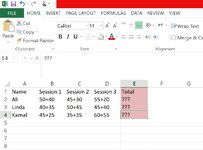
In order to calculate my students' final grade, I have made a spreadsheet like this:

Name I Session 1 I Session 2 I ... I Session 20 I Total

Ali 50+40 45+30 .... 55+20 the Sum Total for Ali???

Linda 40+35 50+45 .... 45+40 the Sum Total for Linda???

Kamal 45+25 35+35 .... 60+55 the Sum Total for Kamal???

As you can see, I give each student 2 grades every session & these two grades must be added together. At the same time, my students & I need to see both numbers which refer to two different marks SEPARATELY (as it is shown above), therefore I can't just enter the summation result in the related cell under each session

Can you please suggest a formula or any solution that will enable me to **calculate the sum total of all the numbers in every row** while I can keep this format of data entry???

P. S. I don't mind changing the addition symbol (+) to a comma (,) between each pair of numbers as long as the OVERALL TOTAL of all entered numbers is correctly calculated.

Appreciate your help very much???

 

[kweaver]

Would you use XL2BB to provide a few examples of your data and what you expect as your result?

 

[kweaver]

Does it look like this? Adjust the ranges based on the number of sessions:

Book2
	A	B	C	D	E	F	G
1	Student	Session 1	Session 2	Session 3		TOTAL-A	TOTAL-B
2	Ali	50+40	45+30	55+20		150+90	240
3	Linda	40+35	50+45	45+40		135+120	255
4	Kamal	45+25	35+35	60+55		140+115	255
Sheet1

Cell Formulas
Range	Formula
F2:F4	F2	=SUM(1*LEFT(B2:D2,FIND("+",B2:D2)-1))&"+"&SUM(1*RIGHT(B2:D2,LEN(B2:D2)-FIND("+",B2:D2)))
G2:G4	G2	=LEFT(F2,FIND("+",F2)-1)+RIGHT(F2,LEN(F2)-FIND("+",F2)+1)
Press CTRL+SHIFT+ENTER to enter array formulas.

 

[excelinmyjob]

Will this Image help??

I'm going to retain the entry format of the numbers the way you see in this picture. Is it possible to calculate the **overall total for every row**, so that I can get 240 as "the total of the first row", 255 as "the total of the second row", and 255 as "the total of the third row"???

Actually, I have to do such calculations for 20 sessions (not just 3 sessions) for every single student! This is why I am counting on excel to do this task for me.

 

[excelinmyjob]

Does it look like this? Adjust the ranges based on the number of sessions:

Book2
	A	B	C	D	E	F	G
1	Student	Session 1	Session 2	Session 3		TOTAL-A	TOTAL-B
2	Ali	50+40	45+30	55+20		150+90	240
3	Linda	40+35	50+45	45+40		135+120	255
4	Kamal	45+25	35+35	60+55		140+115	255
Sheet1

Cell Formulas
Range	Formula
F2:F4	F2	=SUM(1*LEFT(B2:D2,FIND("+",B2:D2)-1))&"+"&SUM(1*RIGHT(B2:D2,LEN(B2:D2)-FIND("+",B2:D2)))
G2:G4	G2	=LEFT(F2,FIND("+",F2)-1)+RIGHT(F2,LEN(F2)-FIND("+",F2)+1)
Press CTRL+SHIFT+ENTER to enter array formulas.

I think you hit the nail on the head

Many thanks dear kweaver???? ?

 

[kweaver]

How's this:

Book2
	A	B	C	D	E	F	G	H	I	J	K	L	M	N	O	P	Q	R	S	T	U	V	W	X
1	Student	Session 1	Session 2	Session 3	Session 4	Session 5	Session 6	Session 7	Session 8	Session 9	Session 10	Session 11	Session 12	Session 13	Session 14	Session 15	Session 16	Session 17	Session 18	Session 19	Session 20		TOTAL-A	TOTAL-B
2	Ali	50+40	45+30	55+20																100+50			250+140	390
3	Linda	40+35	50+45	45+40																			135+120	255
4	Kamal	45+25	35+35	60+55																			140+115	255
Sheet1

Cell Formulas
Range	Formula
W2:W4	W2	=SUM(1*IFERROR(LEFT(B2:U2,FIND("+",B2:U2)-1),0))&"+"&SUM(IFERROR(1*RIGHT(B2:U2,LEN(B2:U2)-FIND("+",B2:U2)),0))
X2:X4	X2	=LEFT(W2,FIND("+",W2)-1)+RIGHT(W2,LEN(W2)-FIND("+",W2)+1)
Press CTRL+SHIFT+ENTER to enter array formulas.

 

[excelinmyjob]

How's this:

Book2
	A	B	C	D	E	F	G	H	I	J	K	L	M	N	O	P	Q	R	S	T	U	V	W	X
1	Student	Session 1	Session 2	Session 3	Session 4	Session 5	Session 6	Session 7	Session 8	Session 9	Session 10	Session 11	Session 12	Session 13	Session 14	Session 15	Session 16	Session 17	Session 18	Session 19	Session 20		TOTAL-A	TOTAL-B
2	Ali	50+40	45+30	55+20																100+50			250+140	390
3	Linda	40+35	50+45	45+40																			135+120	255
4	Kamal	45+25	35+35	60+55																			140+115	255
Sheet1

Cell Formulas
Range	Formula
W2:W4	W2	=SUM(1*IFERROR(LEFT(B2:U2,FIND("+",B2:U2)-1),0))&"+"&SUM(IFERROR(1*RIGHT(B2:U2,LEN(B2:U2)-FIND("+",B2:U2)),0))
X2:X4	X2	=LEFT(W2,FIND("+",W2)-1)+RIGHT(W2,LEN(W2)-FIND("+",W2)+1)
Press CTRL+SHIFT+ENTER to enter array formulas.

Superb!