Hi, so I am building an excel chart and I've tried a few formulas and I can't figure this one out.
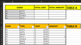
In Cell D3:D6, use a formula that will add up the total costs from TABLE B for the matching code.
In Cell E3:E6, use a formula that will add up the total amounts from TABLE B for the matching code.
Let me know if this sounds confusing. Attached is TABLE A and TABLE B.
In Cell D3:D6, use a formula that will add up the total costs from TABLE B for the matching code.
In Cell E3:E6, use a formula that will add up the total amounts from TABLE B for the matching code.
Let me know if this sounds confusing. Attached is TABLE A and TABLE B.