need help finding cells with different values that contain the same mailing address

[bel85742]

Hello,

I have a large excel sheet of about 40,000 records I've been painfully looking through manually. I sorted the listed by mailing address and used the duplicate values excel function to highlight the duplicate mailing addresses. I don't want to remove the duplicates but what I'm looking for is a way to find the ones that have anything different in the other columns when they have the same mailing address only.

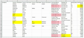
My mailing address is in column F.
Column A is company
Column B is Owner 1 First Name
Column C is Owner 1 Last Name
Column D is Owner 2 First Name
Column E is Owner 2 Last Name
Column G is mailing city
Column H is mailing state
Column I is mailing zip

I made a sample table with examples.
Rows 3 & 4 have the mailing address so I want to compare the other columns in rows 3 & 4 looking for differences in the data. The zip codes are different
Rows 9 & 10 have the mailing address so I want to compare the other columns in rows 9 & 10 looking for differences in the data. The first names are different
Rows 14 & 15 have the mailing address so I want to compare the other columns in rows 14 & 15 looking for differences in the data. The Owner 1 First Name & Owner 2 First Name are different

Ideally I would like to just show the cells that need to be examined and corrected some way by maybe highlighting the records or hiding the good ones

Hope this make sense

Thank you,
Brad

 

[Micron]

Well, if you're up for using vba, one way might be to
- create a 2 dimensional array of range addresses **
- loop over the array and compare (e.g.) F2 & F3. If not identical compare F3 & F4. Rinse and repeat until a match.
- variable i = the 1st row number of a matched pair.
- loop over the array rows as B(i):I(i) and compare to B(i+1):I(i+1) one pair at a time
(e.g.) B3:I3 and compare to B4:I4
If they are not the same, change a cell characteristic (back color, border, whatever)

**I'm no Excel vba expert but I'm pretty sure a two dimensional array of range addresses is a thing and would be the way to go. The alternative might be 2 one dimensional arrays but likely not as efficient, although maybe harder to code. I just don't know how to do it (yet?).

I hope you don't mind me answering in a general sense - I wanted to follow this because I expect someone can code it almost as fast as I can write this post and I'd sure like to see that.

 

[bel85742]

Well, if you're up for using vba, one way might be to
- create a 2 dimensional array of range addresses **
- loop over the array and compare (e.g.) F2 & F3. If not identical compare F3 & F4. Rinse and repeat until a match.
- variable i = the 1st row number of a matched pair.
- loop over the array rows as B(i):I(i) and compare to B(i+1):I(i+1) one pair at a time
(e.g.) B3:I3 and compare to B4:I4
If they are not the same, change a cell characteristic (back color, border, whatever)

**I'm no Excel vba expert but I'm pretty sure a two dimensional array of range addresses is a thing and would be the way to go. The alternative might be 2 one dimensional arrays but likely not as efficient, although maybe harder to code. I just don't know how to do it (yet?).

I hope you don't mind me answering in a general sense - I wanted to follow this because I expect someone can code it almost as fast as I can write this post and I'd sure like to see that.

Hello,

Thanks for providing an idea. I'll look into using an array some more.

 

[Peter_SSs]

Welcome to the MrExcel board!

For the future I suggest that you investigate XL2BB for providing sample data to make it easier for helpers by not having to manually type out sample data to test with. (Then you wouldn't end up with rubbish sample data like mine. )

See if something like this would suit you. Add a 'Check' column like I have in column J and then filter column J for all the '1' values and you will have all the rows that match in column G but have a mis-match somewhere else visible and all the other rows will be hidden.

23 09 07.xlsm
	A	B	C	D	E	F	G	H	I	J
1	Hdr 1	Hdr 2	Hdr 3	Hdr 4	Hdr 5	Hdr 6	Hdr 7	Hdr 8	Hdr 9	Check
2							a
3		x	q				b	p	4	1
4		x	q				b	p	5	1
5							c
6		a	a	a		a	d	222	222
7		a	a	a		a	d	222	222
8							e
9							f
10		Jack					g			1
11		Jill					g			1
12		Jack					g			1
Differences

Cell Formulas
Range	Formula
J2:J12	J2	=IF(ROWS(UNIQUE(FILTER(A$2:I$40000,G$2:G$40000=G2)))>1,1,"")

 

[bel85742]

Welcome to the MrExcel board!

For the future I suggest that you investigate XL2BB for providing sample data to make it easier for helpers by not having to manually type out sample data to test with. (Then you wouldn't end up with rubbish sample data like mine. )

See if something like this would suit you. Add a 'Check' column like I have in column J and then filter column J for all the '1' values and you will have all the rows that match in column G but have a mis-match somewhere else visible and all the other rows will be hidden.

23 09 07.xlsm
	A	B	C	D	E	F	G	H	I	J
1	Hdr 1	Hdr 2	Hdr 3	Hdr 4	Hdr 5	Hdr 6	Hdr 7	Hdr 8	Hdr 9	Check
2							a
3		x	q				b	p	4	1
4		x	q				b	p	5	1
5							c
6		a	a	a		a	d	222	222
7		a	a	a		a	d	222	222
8							e
9							f
10		Jack					g			1
11		Jill					g			1
12		Jack					g			1
Differences

Cell Formulas
Range	Formula
J2:J12	J2	=IF(ROWS(UNIQUE(FILTER(A$2:I$40000,G$2:G$40000=G2)))>1,1,"")

Brilliant. This 1 liner work perfectly. It found all kinds of mistakes I missed. Thank you so much.

 

[Peter_SSs]

You're welcome. Thanks for the follow-up.

 

[Micron]

Never ceases to amaze me what people can do with formulas.