Need to reference rows with a blank cell on another sheet

[CCASSETTY]

I know this is a simple one for regular Excel users, but I'm pretty green at this. All I need to do is reference some data from sheet 1 on sheet 2. Here's what I'm trying to accomplish (screenshot example attached)

SHEET 1
COL A (domain)
COL B (name) Joe Smith
COL C (mailbox name)
COL D (size MB)
COL E (size GB) NUMERICAL VALUE, EX: 1.50

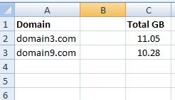
SHEET 2
I need to display [SHEET 1 COL A] and [SHEET 1 COL E] IF [SHEET 1 COL B] is blank.

Unfortunately, the most VBA I know is how to copy what I find on the web, tweak cell ranges, and paste. Can someone tell me how to do this?

Thanks!

 

[hajiali]

Try this in sheet2

Book1
	A	B	C
1	Domain		TOTAL GB
2	domain3.com		11.05
3	domain9.com		10.29
Sheet2

Cell Formulas
Range	Formula
A2:A3	A2	=IFERROR(INDEX(Sheet1!$A$2:$A$10,AGGREGATE(15,6,(ROW(Sheet1!$A$2:$A$10)-ROW(Sheet1!$A$2)+1)/(Sheet1!$B$2:$B$10=""),ROWS(Sheet1!$A$2:A2))),"")
C2:C3	C2	=IFERROR(INDEX(Sheet1!$E$2:$E$10,MATCH(A2,Sheet1!$A$2:$A$10,0)),"")

 

[BigBeachBananas]

You need to adjust the cell ranges, but how about this:

Book1
	A	B	C	D	E	F	G	H	I	J	K
1	Domain	UserName	q	Size(MB)	Size(GB)				Domain		Size(GB)
2	Domain1			10378	10.8978344				Domain1		10.89783
3	Domain2	xx		11318	10.93766136				Domain4		10.92796
4	Domain3	xx	main	10475	10.90956863				Domain5		10.27375
5	Domain4			10942	10.92796073				Domain6		10.865
6	Domain5			10160	10.27374883				Domain8		10.24031
7	Domain6			10864	10.865004				Domain9		10.9588
8	Domain7	xxxx	main	10534	10.25278495
9	Domain8			10056	10.24031221
10	Domain9			10711	10.78806729
11	Domain10	xx		10721	10.96089124
12	Domain11	x		11401	10.95880298
Sheet3

Cell Formulas
Range	Formula
I2:I7	I2	=FILTER(A2:A12,ISBLANK(B2:B12)=TRUE)
K2:K7	K2	=VLOOKUP(I2,A1:E12,5)
Dynamic array formulas.

 

[CCASSETTY]

You need to adjust the cell ranges, but how about this:

Book1
	A	B	C	D	E	F	G	H	I	J	K
1	Domain	UserName	q	Size(MB)	Size(GB)				Domain		Size(GB)
2	Domain1			10378	10.8978344				Domain1		10.89783
3	Domain2	xx		11318	10.93766136				Domain4		10.92796
4	Domain3	xx	main	10475	10.90956863				Domain5		10.27375
5	Domain4			10942	10.92796073				Domain6		10.865
6	Domain5			10160	10.27374883				Domain8		10.24031
7	Domain6			10864	10.865004				Domain9		10.9588
8	Domain7	xxxx	main	10534	10.25278495
9	Domain8			10056	10.24031221
10	Domain9			10711	10.78806729
11	Domain10	xx		10721	10.96089124
12	Domain11	x		11401	10.95880298
Sheet3

Cell Formulas
Range	Formula
I2:I7	I2	=FILTER(A2:A12,ISBLANK(B2:B12)=TRUE)
K2:K7	K2	=VLOOKUP(I2,A1:E12,5)
Dynamic array formulas.

Unfortunately, this won't work for me, as I see this is only supported in the (much) newer versions than what I'm stuck working with. But thank you.

 

[CCASSETTY]

Try this in sheet2

Book1
	A	B	C
1	Domain		TOTAL GB
2	domain3.com		11.05
3	domain9.com		10.29
Sheet2

Cell Formulas
Range	Formula
A2:A3	A2	=IFERROR(INDEX(Sheet1!$A$2:$A$10,AGGREGATE(15,6,(ROW(Sheet1!$A$2:$A$10)-ROW(Sheet1!$A$2)+1)/(Sheet1!$B$2:$B$10=""),ROWS(Sheet1!$A$2:A2))),"")
C2:C3	C2	=IFERROR(INDEX(Sheet1!$E$2:$E$10,MATCH(A2,Sheet1!$A$2:$A$10,0)),"")

I'm afraid I'm not astute enough to follow because I've tried and I'm obviously doing something wrong. I apologize, but could you explain it like I'm five?

 

[hajiali]

I'm afraid I'm not astute enough to follow because I've tried and I'm obviously doing something wrong. I apologize, but could you explain it like I'm five?

so what I did was copy that formula

=IFERROR(INDEX(Sheet1!$A$2:$A$10,AGGREGATE(15,6,(ROW(Sheet1!$A$2:$A$10)-ROW(Sheet1!$A$2)+1)/(Sheet1!$B$2:$B$10=""),ROWS(Sheet1!$A$2:A2))),"")

to sheet2 in cell A2 and drag it down.

I only went down to Sheet1 cell Row 10 in the formula put you can put whatever row number you need just change "10" to the row number in the formula

Sheet1!$A$2:$A$10)

then I put

IFERROR(INDEX(Sheet1!$E$2:$E$10,MATCH(A2,Sheet1!$A$2:$A$10,0)),"")

In sheet2 in cell C2 and drag that down. again I only went with 10 rows for the example

Hope that clears and helps