Need to return first non-blank cell based in one column on a date in another column.

[excelcpa95]

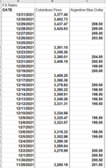
I have a spreadsheet that has a bunch of exchange rates with dates in Column A (most recent date at the top) and exchange rates in the rest of the columns.

I previously used INDEX/MATCH to look up exchange rates on specific dates or the average of exchange rates over a date range. Unfortunately, I have recently integrated some currencies that do not have an exchange rate value for every date, but has a handful of blank cells. I want to lookup so that if the specific date I am looking up is blank, it will return the next non-blank value for the most recent date with a value prior to the date that has a blank cell.

Under my current formulas, I use the array as my INDEX reference, and MATCH Functions using the Date as the Row_Num and Currency as the Column_Num.

How would I be able to accomplish this?

 

[Toadstool]

Hi Excelcpa95,

As long as your dates remain in latest first sequence then this should work.

Excelcpa95.xlsx
	A	B	C	D	E	F	G	H
1	FX Rate				Date=	19-Dec-21	Currency=	Argentine Blue Dollar
2	Date	Colombian Peso	Argentine Blue Dollar
3	31-Dec-21	3000.00			Result=	246.24
4	30-Dec-21	3060.00
5	29-Dec-21	3121.20	210.16
6	28-Dec-21	3183.62	214.36
7	27-Dec-21		218.65
8	26-Dec-21		223.02
9	25-Dec-21
10	24-Dec-21	3446.06
11	23-Dec-21	3514.98
12	22-Dec-21	3585.28	241.41
13	21-Dec-21	3656.98	246.24
14	20-Dec-21
15	19-Dec-21
16	18-Dec-21	3880.82	261.31
17	17-Dec-21	3958.44	266.53
18	16-Dec-21	4037.61	271.87
Sheet1

Cell Formulas
Range	Formula
F3	F3	=INDEX($B$3:$C$18,AGGREGATE(14,6,ROW($A$3:$A$18)-ROW($A$2)/(($A$3:$A$18>=$F$1)*($B$2:$C$2=$H$1)*($B$3:$C$18<>"")),1),MATCH($H$1,$B$2:$C$2,0))

 

[BSALV]

i used a named range for the dates

Map1
	B	C	D	E	F
1
2				02/05/2022	1006
3	02/08/2022	1096		02/04/2022	1047
4	02/07/2022	1062		02/03/2022	1047
5	02/06/2022	1024		02/02/2022	1047
6	02/05/2022	1006		02/01/2022	1047
7	02/04/2022			01/31/2022	1047
8	02/03/2022			01/30/2022	1047
9	02/02/2022			01/29/2022	1040
10	02/01/2022			01/28/2022	1012
11	01/31/2022			01/27/2022	1004
12	01/30/2022	1047		01/26/2022	1068
13	01/29/2022	1040		01/25/2022	1089
14	01/28/2022	1012		01/24/2022	1089
15	01/27/2022	1004		01/23/2022	1089
16	01/26/2022	1068		01/22/2022	1089
17	01/25/2022
18	01/24/2022
19	01/23/2022
20	01/22/2022
21	01/21/2022
22	01/20/2022	1089
23	01/19/2022	1076
24	01/18/2022	1040
25	01/17/2022	1099
26	01/16/2022	1022
27	01/15/2022
28
29
Blad1

Cell Formulas
Range	Formula
F2:F16	F2	=VLOOKUP(MAX((MyDates<=E2)*(OFFSET(MyDates,,1,,)<>"")*MyDates),OFFSET(MyDates,,,,2),2,0)
E3:E16	E3	=+E2-1

Named Ranges
Name	Refers To	Cells
MyDates	=Blad1!$B$3:$B$27	F2:F16